2D Features framework

https://docs.opencv.org/3.4/d9/d97/tutorial_table_of_content_features2d.html

Feature detection and description are the basis for image recognition and detection. They are especially useful for simple tasks, when there is too few data to train a deep learning model or too little compute power.

Features detector

Harris Corner Detector

Shi-Tomasi

Corner with SubPixel Accuracy

Scale Invariance Feature Transform: (SIFT)

Speed-Up Robust Feature (SURF)

Features from Accelerated Segment Test (FAST)

Features descriptor

Binary Robust Independent Elementary Features (BRIEF)

Oriented FAST and rotated BRIEF (ORB)

Feature Matcher

Homography

Features detector

Harris Corner Detector

https://opencv24-python-tutorials.readthedocs.io/en/latest/py_tutorials/py_feature2d/py_features_harris/py_features_harris.html

A feature should be uniquely recognizable, and can be edges, corners (aka interest points) blob (aka regions of interest)

high variations in image gradient can be use to detect corners

We look for variation of

S(u,v)=∑x∑yw(x,y)[I(x+u,y+v)−I(x,y)]2S(u,v)=\sum_x\sum_yw(x,y)[I(x+u,y+v)-I(x,y)]^2S(u,v)=∑x​∑y​w(x,y)[I(x+u,y+v)−I(x,y)]2﻿​

Using Taylor decomposition, with Ix,IyI_x,I_yIx​,Iy​﻿ partial derivative 

S(u,v)≈∑x∑yw(x,y)[I(x,y)+uIx+vIy−I(x,y)]2S(u,v)\approx\sum_x\sum_yw(x,y)[I(x,y)+uI_x+vI_y-I(x,y)]^2\\S(u,v)≈∑x​∑y​w(x,y)[I(x,y)+uIx​+vIy​−I(x,y)]2﻿​

=∑x∑yw(x,y)(u2Ix2+v2Iy2+2uvIxIy)=\sum_x\sum_yw(x,y)(u^2I_x^2+v^2I_y^2+2uvI_xI_y)\\=∑x​∑y​w(x,y)(u2Ix2​+v2Iy2​+2uvIx​Iy​)﻿​

=[u,v](∑x,yw(x,y)[Ix2IxIyIxIyIy2])[uv]=[u,v]\Big(\sum_{x,y} w(x,y)\begin{bmatrix}I^2_x &I_xI_y \\ I_xI_y & I_y^2\end{bmatrix}
\Big)\begin{bmatrix} u \\ v\end{bmatrix}=[u,v](∑x,y​w(x,y)[Ix2​Ix​Iy​​Ix​Iy​Iy2​​])[uv​]﻿​

=[u,v]M[uv]=[u,v]M\begin{bmatrix}u \\ v\end{bmatrix}=[u,v]M[uv​]﻿​

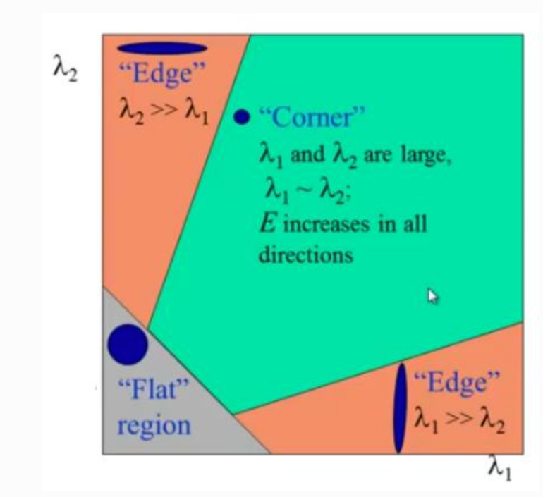
We look at the score R=det(M)−kTr(M)=λ1λ2−k(λ1+λ2)R=det(M)-kTr(M)=\lambda_1\lambda_2-k(\lambda_1+\lambda_2)R=det(M)−kTr(M)=λ1​λ2​−k(λ1​+λ2​)﻿​

with λ1,λ2\lambda_1,\lambda_2λ1​,λ2​﻿ eigenvalues of M

A window with a high RRR﻿ is considered a corner

If λ1≈0\lambda _{1}\approx 0λ1​≈0﻿ and λ2\lambda _{2}λ2​﻿ has some large positive value, then an edge is found.

If λ1\lambda _{1}λ1​﻿ and λ2\lambda _{2}λ2​﻿ have large positive values, then a corner is found.

Exact computation of the eigenvalues is computationally expensive, since it requires the computation of a square root, hence the RRR﻿ equation

Python

Copy

dst = cv2.cornerHarris(gray, blockSize=2, apertureSize=3, k=0.04)

dst_norm = np.empty(dst.shape, dtype=np.float32)
cv.normalize(dst, dst_norm, alpha=0, beta=255, norm_type=cv.NORM_MINMAX)
dst_norm_scaled = cv.convertScaleAbs(dst_norm)
# Drawing a circle around corners
for i in range(dst_norm.shape[0]):
for j in range(dst_norm.shape[1]):
if int(dst_norm[i,j]) > thresh:
            cv.circle(dst_norm_scaled, (j,i), 5, (0), 2)
# or
#result is dilated for marking the corners, not important
dst = cv2.dilate(dst,None)
# Threshold for an optimal value, it may vary depending on the image.
img[dst>0.01*dst.max()]=[0,0,255]

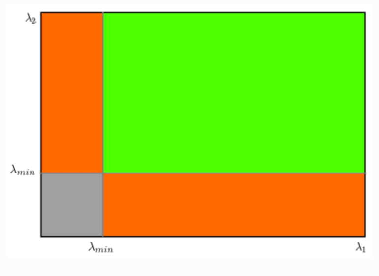
Shi-Tomasi

Propose instead the score R=min(λ1,λ2)R=min(\lambda_1,\lambda_2)R=min(λ1​,λ2​)﻿​

Arduino

Copy

corners = cv2.goodFeaturesToTrack(
	src_gray,
	maxCorners,
	qualityLevel=0.01,
	minDistance=10,
	None,
  blockSize=3,
	gradientSize=3,
	useHarrisDetector=False,
	k=0.04
)

corners = np.int0(corners)
for i in corners:
    x,y = i.ravel()
    cv2.circle(img,(x,y),3,255,-1)

This function is more appropriate for tracking

Corner with SubPixel Accuracy

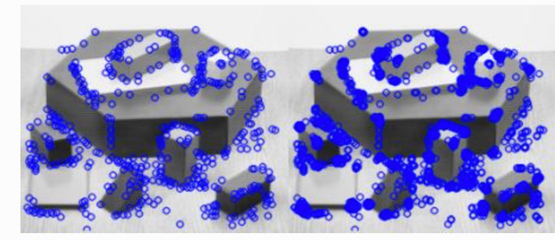
https://opencv24-python-tutorials.readthedocs.io/en/latest/py_tutorials/py_feature2d/py_features_harris/py_features_harris.html#corner-with-subpixel-accuracy

Find the corners with maximum accuracy

Python

Copy

dst = cv2.cornerHarris(gray,2,3,0.04)
dst = cv2.dilate(dst,None)
ret, dst = cv2.threshold(dst,0.01*dst.max(),255,0)
dst = np.uint8(dst)
# find centroids
ret, labels, stats, centroids = cv2.connectedComponentsWithStats(dst)
# define the criteria to stop and refine the corners
criteria = (cv2.TERM_CRITERIA_EPS + cv2.TERM_CRITERIA_MAX_ITER, 100, 0.001)
corners = cv2.cornerSubPix(gray,np.float32(centroids),(5,5),(-1,-1),criteria)
# Now draw them
res = np.hstack((centroids,corners))
res = np.int0(res)
img[res[:,1],res[:,0]]=[0,0,255]
img[res[:,3],res[:,2]] = [0,255,0]

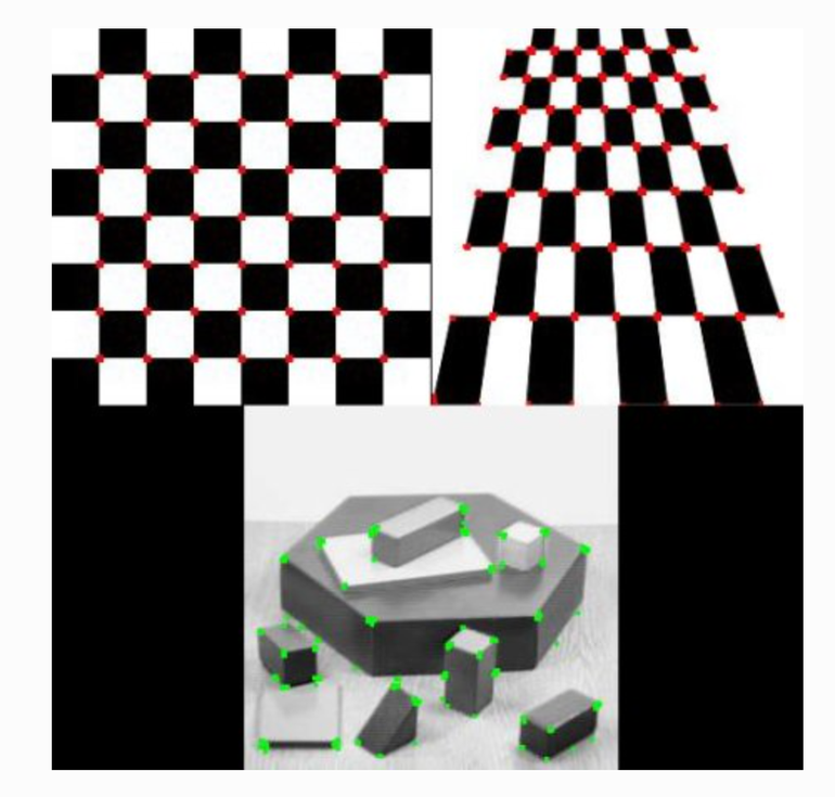
Find the Harris Corners

Pass the centroids of these corners (There may be a bunch of pixels at a corner, we take their centroid) to refine them. 

Harris corners are marked in red pixels and refined corners are marked in green pixels. For this function, we have to define the criteria when to stop the iteration. We stop it after a specified number of iteration or a certain accuracy is achieved, whichever occurs first. 

We also need to define the size of neighbourhood it would search for corners.

Scale Invariance Feature Transform: (SIFT)

https://opencv24-python-tutorials.readthedocs.io/en/latest/py_tutorials/py_feature2d/py_sift_intro/py_sift_intro.html#introduction-to-sift-scale-invariant-feature-transform

Harris and Shi-Tomasi corner detectors are rotation invariant(an edge remains an edge) but not scale invariant (zooming on an edge so that you can't detect it)

SIFT extract keypoints and compute its descriptor

Scale-space Extrema Detection

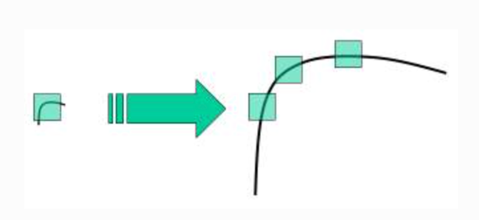
To detect larger corner we need larger windows

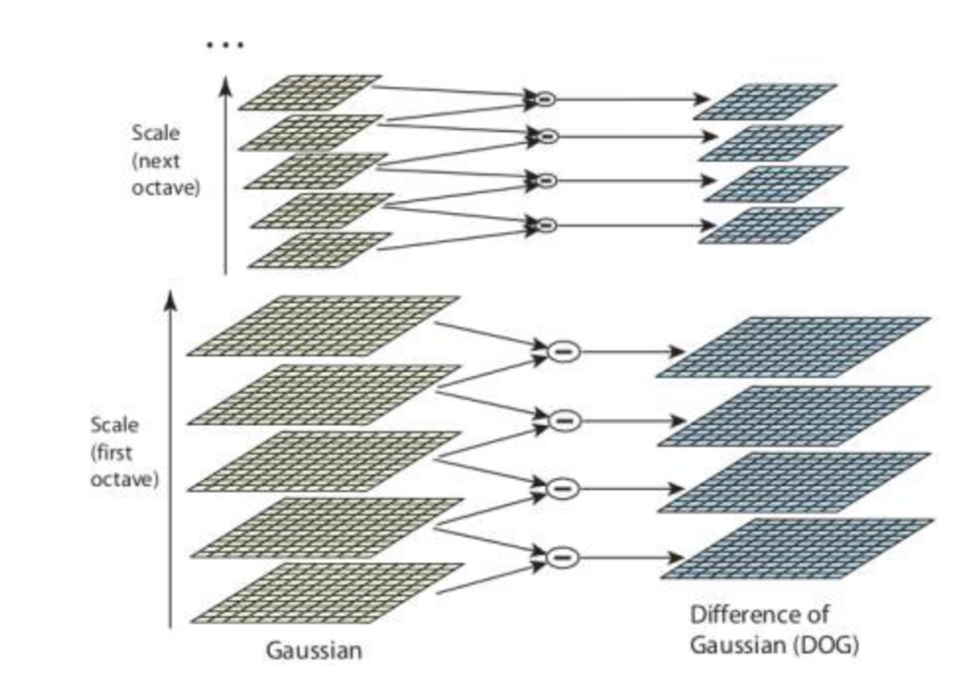
Laplacian of Gaussian (LoG) acts as a blob detector which detects blobs in various sizes, σ\sigma σ﻿ acts as a scaling parameter (large σ\sigmaσ﻿ to detect large corner)

We can find local maxima across the scale and space, to find potential keypoints at (x,y)(x, y)(x,y)﻿ at scale σ\sigmaσ﻿​

But costly in compute, so use an approximation: Difference of Gaussians (DoG), consists in computing difference between two Gaussian blur with different σ\sigmaσ﻿​

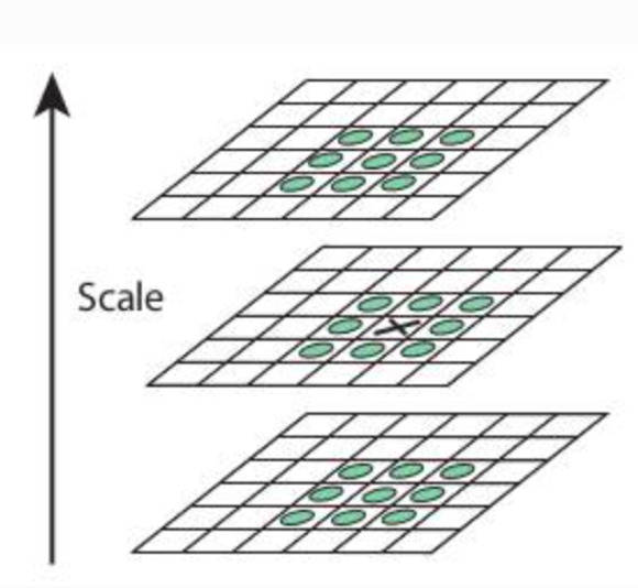
We compare at given pixel it to its 8 neighbours, along with previous and next scale. If its an local extrema, (x,y,σ)(x, y,\sigma)(x,y,σ)﻿ is a potential keypoint

Keypoint Localization

Need to remove both low contrast keypoints and edge keypoints so that only strong interests keypoints remain

Taylor series expansion of scale space to get more accurate location of extrema

D(x)=D+x∂D∂x+x22∂2D∂2xD(x)=D+x \frac{\partial D}{\partial x} +\frac{x^2}{2}\frac{\partial^2D}{\partial ^2x}D(x)=D+x∂x∂D​+2x2​∂2x∂2D​﻿​

If the intensity of the extrema is below a contrastThreshold, the keypoint is discarded as low-contrast

DoG has higher response for edges even if the candidate keypoint is not robust to small amounts of noise. 

So similarly to Harris detection we compute the ratio between eigenvalues of hessian matrix.

For poorly defined peaks in the DoG function, the principal curvature across the edge would be much larger than the principal curvature along it

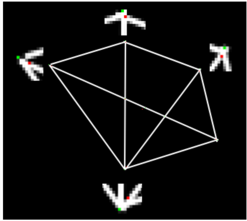
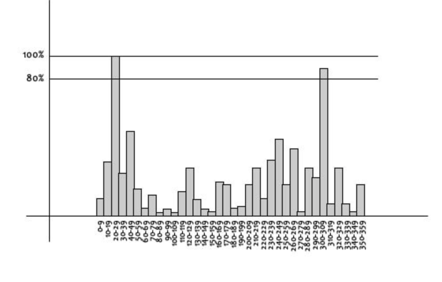
H=[DxxDxyDxyDyy]\bold{H}=\begin{bmatrix} D_{xx} & D_{xy} \\ D_{xy} & D_{yy} \end{bmatrix}H=[Dxx​Dxy​​Dxy​Dyy​​]﻿ and we reject Tr(H)2Det(H)>rth=10\frac{Tr(H)^2}{Det(H)}>r_{th}=10Det(H)Tr(H)2​>rth​=10﻿​

Orientation Assignment

Assign an orientation to each keypoint to achieve image rotation invariance, and improve stability of matching

An orientation histogram with 36 beans covering 360 degree is computed, weighted by gradient magnitude and gaussian circular windows with a scale of 1.5 the scale of keypoint

m(x,y)=(L(x+1,y)−L(x−1,y))2+(L(x,y+1)−L(x,y−1))2m(x,y)=\sqrt{(L(x+1,y)-L(x-1,y))^2+(L(x,y+1)-L(x,y-1))^2}m(x,y)=(L(x+1,y)−L(x−1,y))2+(L(x,y+1)−L(x,y−1))2​﻿​

θ(x,y)=atan2(L(x,y+1)−L(x,y−1),L(x+1,y)−L(x−1,y)){\displaystyle \theta \left(x,y\right)=\mathrm {atan2} \left(L\left(x,y+1\right)-L\left(x,y-1\right),L\left(x+1,y\right)-L\left(x-1,y\right)\right)}θ(x,y)=atan2(L(x,y+1)−L(x,y−1),L(x+1,y)−L(x−1,y))﻿​

We consider all peak above 80% of the histogram to compute orientation

Keypoint Descriptor

Our goal is now to compute a descriptor for the local image region about each keypoint that is highly distinctive and invariant as possible to variations such as changes in viewpoint and illumination.

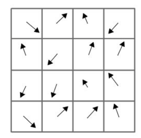
We split a 16x16 neighborhood into 16 sub-blocks of 4x4 size

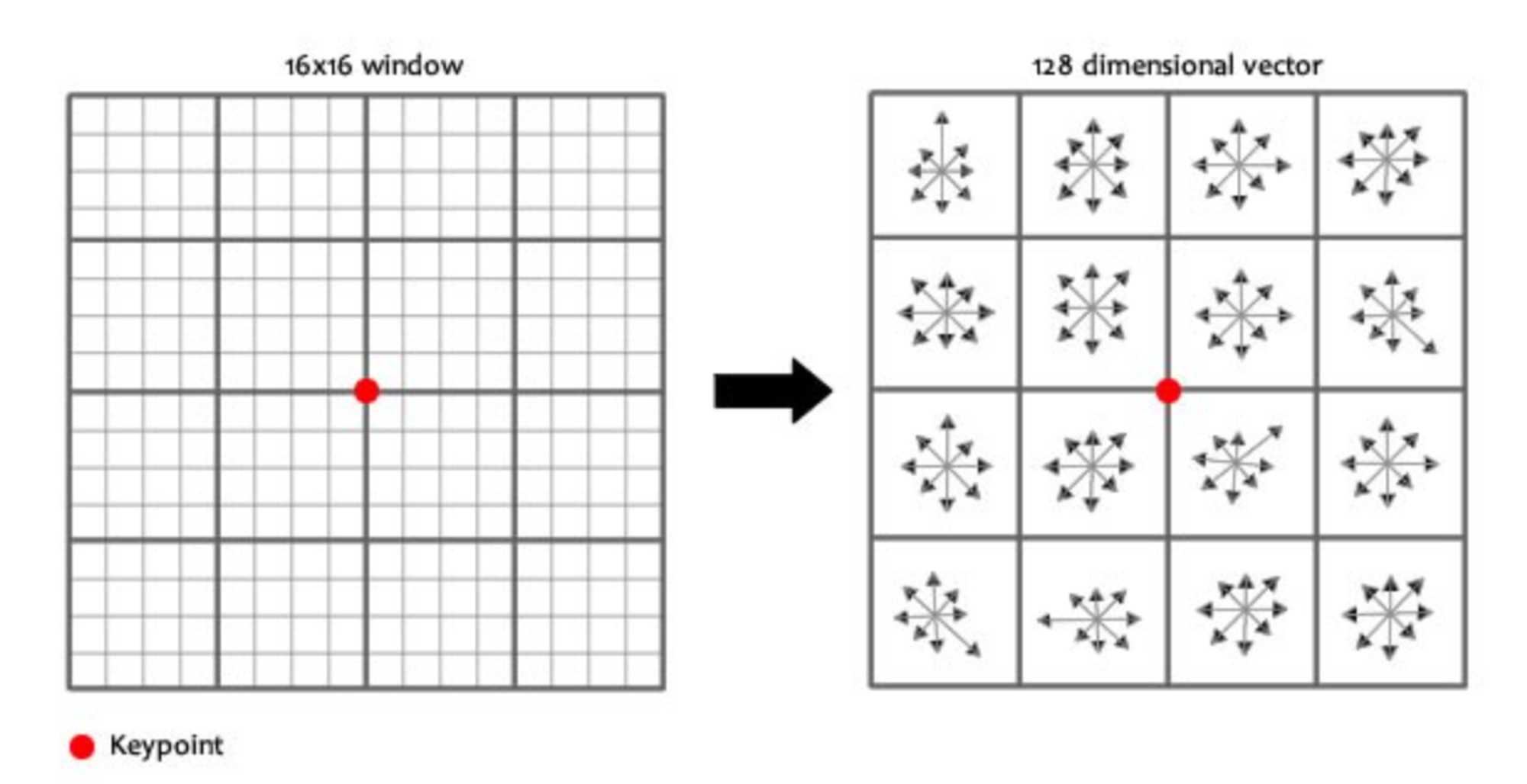
Create 8 bin orientation histogram for each sub-block, that's a 128 bin descriptor vector in total

This vector is then normalized to unit length in order to enhance invariance to affine changes in illumination.

Implementation

Python

Copy

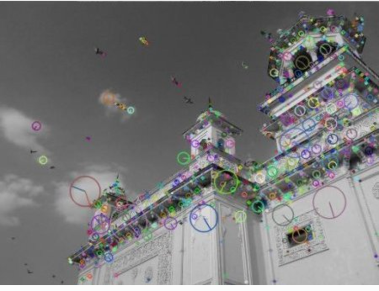
sift = cv2.SIFT()
kp = sift.detect(gray, None)

img = cv2.drawKeypoints(
		gray,
		kp,
		flags=cv2.DRAW_MATCHES_FLAGS_DRAW_RICH_KEYPOINTS
)

or compute keypoints, descriptor  directly

Python

Copy

sift = cv2.SIFT()
kp, des = sift.detectAndCompute(gray,None)

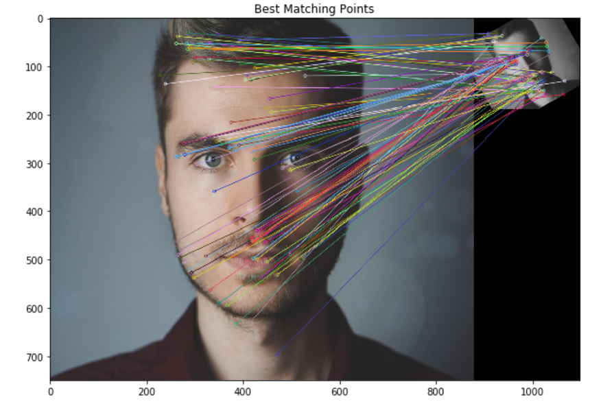
Keypoints matching

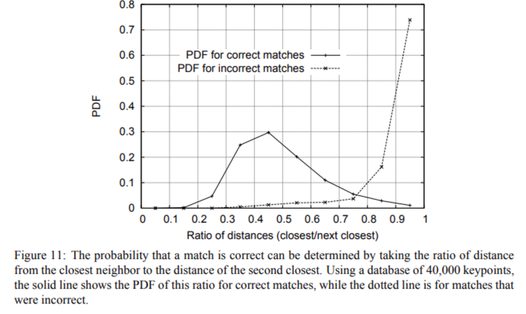
Keypoints between two images are matched by identifying their nearest neighbours

In some case, the second-closest match is very near to the first (due to noise)

We eliminate first/second ratio higher than 0.8, it eliminates 90% of false positive and only 5% of true positive

Speed-Up Robust Feature (SURF)

https://docs.opencv.org/3.4/d7/d66/tutorial_feature_detection.html

https://opencv24-python-tutorials.readthedocs.io/en/latest/py_tutorials/py_feature2d/py_surf_intro/py_surf_intro.html#surf

https://medium.com/data-breach/introduction-to-surf-speeded-up-robust-features-c7396d6e7c4e

Composed of feature extraction + feature description

SIFT but faster

Feature extraction

Instead of computing Laplacian of Gaussian (LoG) using Difference of Gaussian (DoG) we approximate using box filter

We smooth the image and take gaussian second order derivative, and this is approximated via boxes below:

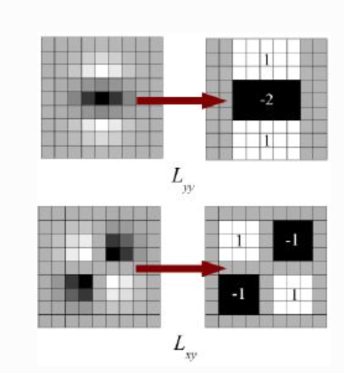
Instead of computing the determinant of the Hessian Matrix

H(x,σ)=[Lxx(x,σ)Lxy(x,σ)Lxy(x,σ)Lyy(x,σ)]H(\bold{x},\sigma)=\begin{bmatrix} L_{xx}(\bold{x},\sigma) & L_{xy}(\bold{x},\sigma) \\ L_{xy}(\bold{x},\sigma) & L_{yy}(\bold{x},\sigma) \end{bmatrix}H(x,σ)=[Lxx​(x,σ)Lxy​(x,σ)​Lxy​(x,σ)Lyy​(x,σ)​]﻿​

We multiply the image through the box approximation, yielding the following determinant

Det(Happrox)=DxxDyy−(wDxy2)Det(H_{approx})=D_{xx}D_{yy}-(wD_{xy}^2)Det(Happrox​)=Dxx​Dyy​−(wDxy2​)﻿, with w=0.9w=0.9w=0.9﻿​

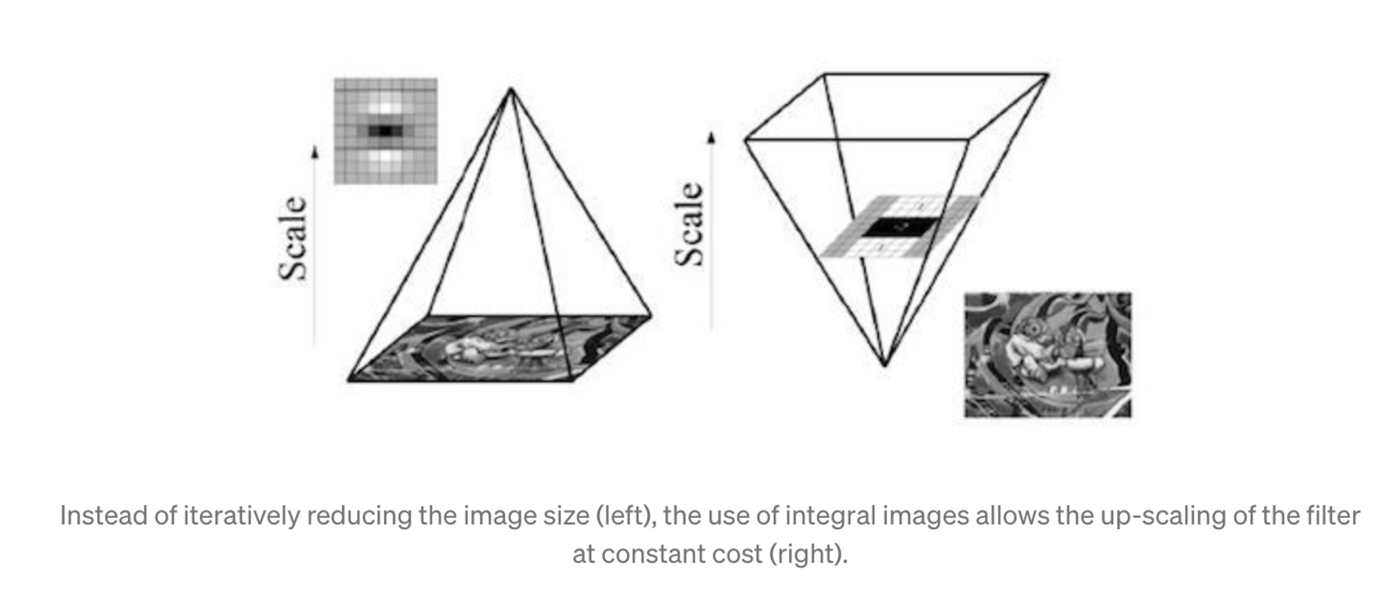
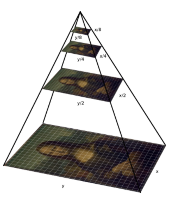
Scale-space are represented as pyramids, and instead of reducing the image size, we increase the filter size

For feature description, SURF uses Wavelet responses in horizontal and vertical direction (again, use of integral images makes things easier)

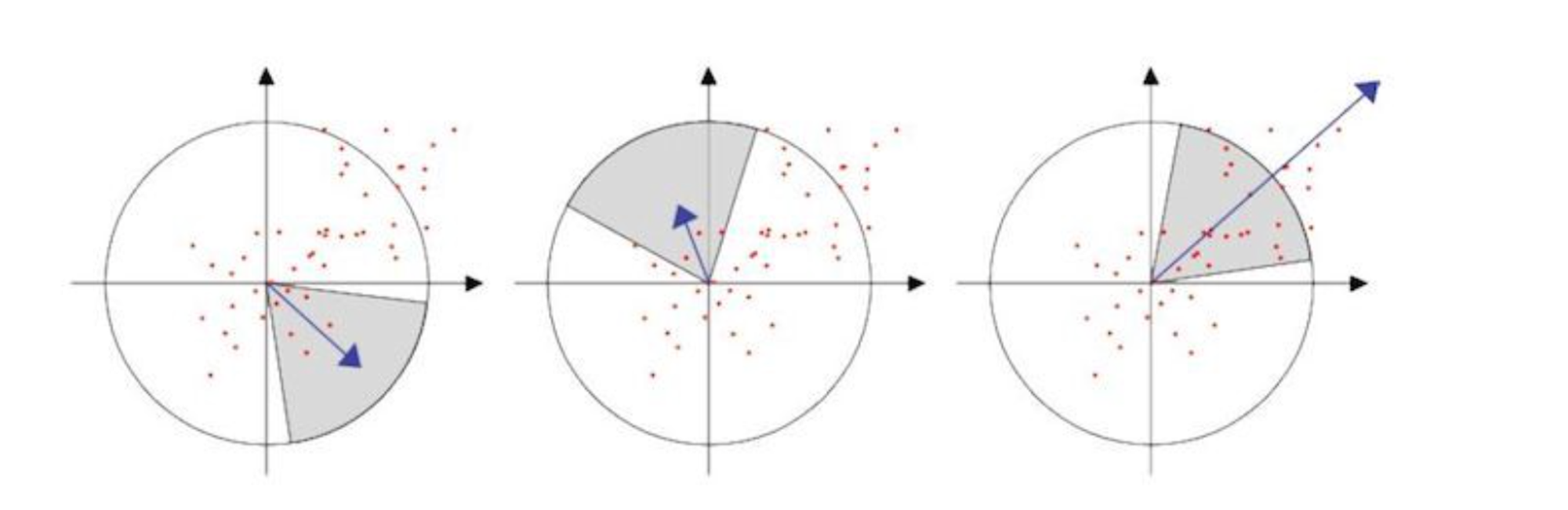
Orientation assignment

by computing Haar Wavelet on x and y direction in a scale dependant circular radius neighborhood of 6s of the detected keypoint

Iteratively compute the sum of vertical and horizontal wavelet response in the area, and change area orientation by +π/3+ \pi/3+π/3﻿​

This orientation with the largest sum is our main one for the feature descriptor

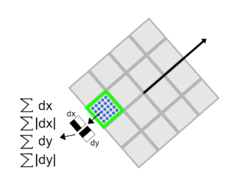
Descriptor components

Create window of size 20s centered around keypoint using its orientation

Split into 16 regions of size 5s each, and compute Haar wavelet in x (dx) and y (dy), filter size of 2s. Responses are weighted by Gaussian centered at keypoint.

Build our size 64 vector by computing the 4 components for each region (vs size 128 for SIFT, hence its speed)

SURF is good at handling images with blurring and rotation, but not good at handling viewpoint change and illumination change.

Python

Copy

# Create SURF object. You can specify params here or later.
# Here I set Hessian Threshold to 400
surf = cv2.SURF(400)
# Find keypoints and descriptors directly
kp, des = surf.detectAndCompute(img, None)
# len(kp) gives 1199 points, too much to show in a picture.
# We reduce it to some 50 to draw it on an image.
# While matching, we may need all those features, but not now.
# So we increase the Hessian Threshold.
# We set it to some 50000. Remember, it is just for representing in picture.
# In actual cases, it is better to have a value 300-500
surf.hessianThreshold = 50000
# Again compute keypoints and check its number.
kp, des = surf.detectAndCompute(img, None)
# print(len(kp)) gives 47
img2 = cv2.drawKeypoints(img, kp, None, (255, 0, 0), 4)

plt.imshow(img2)

Python

Copy

surf.upright = True

setting upright True is even faster

Python

Copy

# Find size of descriptor
>>> print(surf.descriptorSize())
64
# That means flag, "extended" is False.
>>> surf.extended
 False
# So we make it to True to get 128-dim descriptors.
>>> surf.extended = True
>>> kp, des = surf.detectAndCompute(img,None)
>>> print(surf.descriptorSize())
128
>>> print(des.shape)
(47, 128)

Features from Accelerated Segment Test (FAST)

https://opencv24-python-tutorials.readthedocs.io/en/latest/py_tutorials/py_feature2d/py_fast/py_fast.html

Previous feature detector aren't fast enough for real-time computation, like for SLAM (Simultaneous Localization and Mapping) mobile robot which have limited computational resources

Method

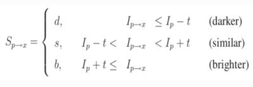
Choose a pixel p, whose intensity is IpI_pIp​﻿​

Select a threshold value ttt﻿​

Take a circle of 16 pixels around p

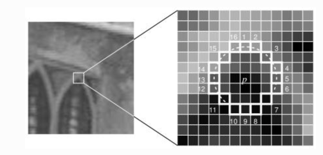
p is a corner if there exists a set of nnn﻿ contiguous point whose intensity are below Ip−tI_p-tIp​−t﻿ or above Ip+tI_p+tIp​+t﻿. Let's choose n=12n=12n=12﻿​

High speed test by looking only at pixels 111﻿ and 999﻿, then 555﻿ and 131313﻿, then full segment criterion (in order to eliminate candidate and process faster)

Shortfalls

Does reject as many candidates for n<12n<12n<12﻿​

Efficiency of the pixels choice depends on distribution of corner appearance and questions ordering

Results of high speed test are thrown away

Multiple features are detected adjacent to each other

Machine learning (shortfall 1-3)

Select a set of images for training

Run FAST algorithm on every images to find feature points

For every feature point, store the 16 pixels surrounding as a vector. It gives a vector P\bold{P}P﻿ for all images

Each pixel x can be in either state

Select x to split the vector into Pd,PsP_d,P_sPd​,Ps​﻿ and PbP_bPb​﻿​

Define a new boolean variable KpK_pKp​﻿, True if ppp﻿ is a corner, False otherwise

Use a ID3 algorithm (decision tree classifier) to find the next pixel number (among 16) until the entropy is 0

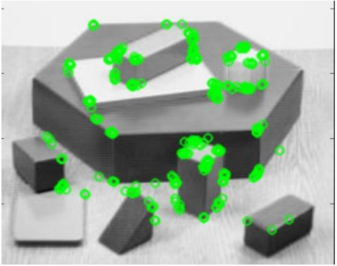
Non maximal suppression (shortfall 4)

Compute Vp=∑i=116∣p−pi∣V_p=\sum_{i=1}^{16} |p-p_i|Vp​=∑i=116​∣p−pi​∣﻿ for all detected feature points

Consider 2 adjacent keypoints, keep the one with the highest VVV﻿​

Still shortfalls

Not robust to high level of noise

Dependent on a threshold

Implementation

Python

Copy

# Initiate FAST object with default values
fast = cv2.FastFeatureDetector_create()
# find and draw the keypoints
kp = fast.detect(img, None)
img2 = cv2.drawKeypoints(img, kp, color=(255, 0, 0))
# Print all default params
print "Threshold: ", fast.getInt('threshold')
print "nonmaxSuppression: ", fast.getBool('nonmaxSuppression')
print "neighborhood: ", fast.getInt('type')
print "Total Keypoints with nonmaxSuppression: ", len(kp)

cv2.imwrite('fast_true.png', img2)

With and without non max suppression

Features descriptor

Binary Robust Independent Elementary Features (BRIEF)

https://opencv24-python-tutorials.readthedocs.io/en/latest/py_tutorials/py_feature2d/py_brief/py_brief.html

https://medium.com/data-breach/introduction-to-brief-binary-robust-independent-elementary-features-436f4a31a0e6

Advantages

Small number of intensity difference tests to represent an image (low memory consumption)

Bulding and matching is faster

Higher recognition rates (but not rotational invariant)

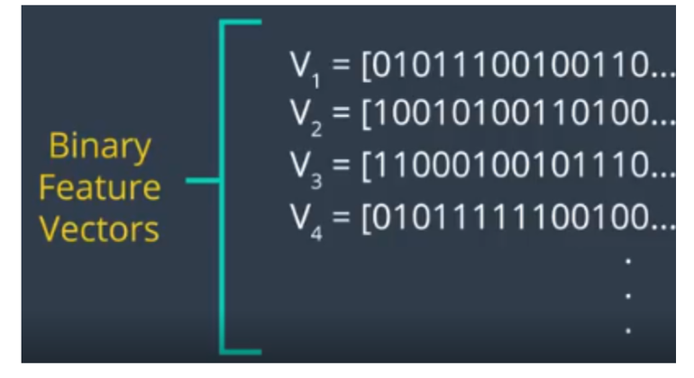
Feature descriptors encode detected keypoints, by converting patch of the pixel neighborhood into binary feature vectors (128–512 bits)

As it focus on the pixel level, BRIEF is super noise sensitive, so Gaussian smoothing is needed

We need to define a set of nnn﻿ pairs within the patch of each keypoint, using of of the below sampling geometries

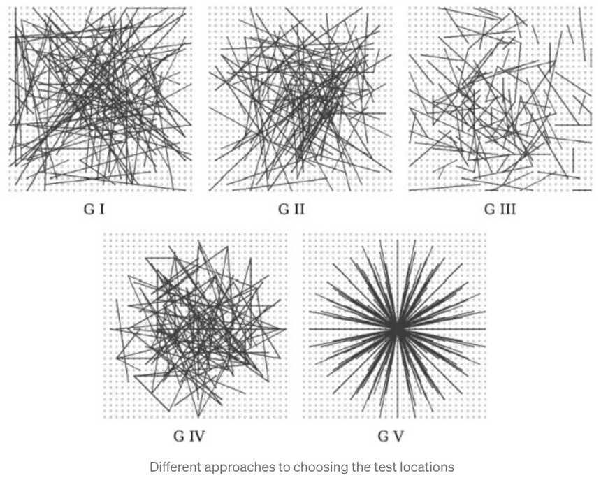
Our BRIF descriptor is fnd(p)=∑1≤i≤nd2i−1τ(p,xi,yi)f_{n_d}(p)=\sum_{1\le i\le n_d} 2^{i-1} \tau (p,x_i,y_i)fnd​​(p)=∑1≤i≤nd​​2i−1τ(p,xi​,yi​)﻿​

with τ(p,xi,yi)={1  if  p(xi)<p(yi)0  o.w.\tau(p,x_i,y_i)=\begin{cases} 1 \;if \;p(x_i)<p(y_i)\\0 \;o.w.\end{cases}τ(p,xi​,yi​)={1ifp(xi​)<p(yi​)0o.w.​﻿ and ppp﻿ the pixel intensity

Implementation

Python

Copy

training_image = cv2.cvtColor(image1, cv2.COLOR_BGR2RGB)
# Convert the training image to gray scale
training_gray = cv2.cvtColor(training_image, cv2.COLOR_RGB2GRAY)
# Create test image by adding Scale Invariance and Rotational Invariance
test_image = cv2.pyrDown(training_image)
test_image = cv2.pyrDown(test_image)
num_rows, num_cols = test_image.shape[:2]

rotation_matrix = cv2.getRotationMatrix2D((num_cols/2, num_rows/2), 30, 1)
test_image = cv2.warpAffine(test_image, rotation_matrix, (num_cols, num_rows))

test_gray = cv2.cvtColor(test_image, cv2.COLOR_RGB2GRAY)

fast = cv2.FastFeatureDetector_create() 
brief = cv2.xfeatures2d.BriefDescriptorExtractor_create()

train_keypoints = fast.detect(training_gray, None)
test_keypoints = fast.detect(test_gray, None)

train_keypoints, train_descriptor = brief.compute(training_gray, train_keypoints)
test_keypoints, test_descriptor = brief.compute(test_gray, test_keypoints)

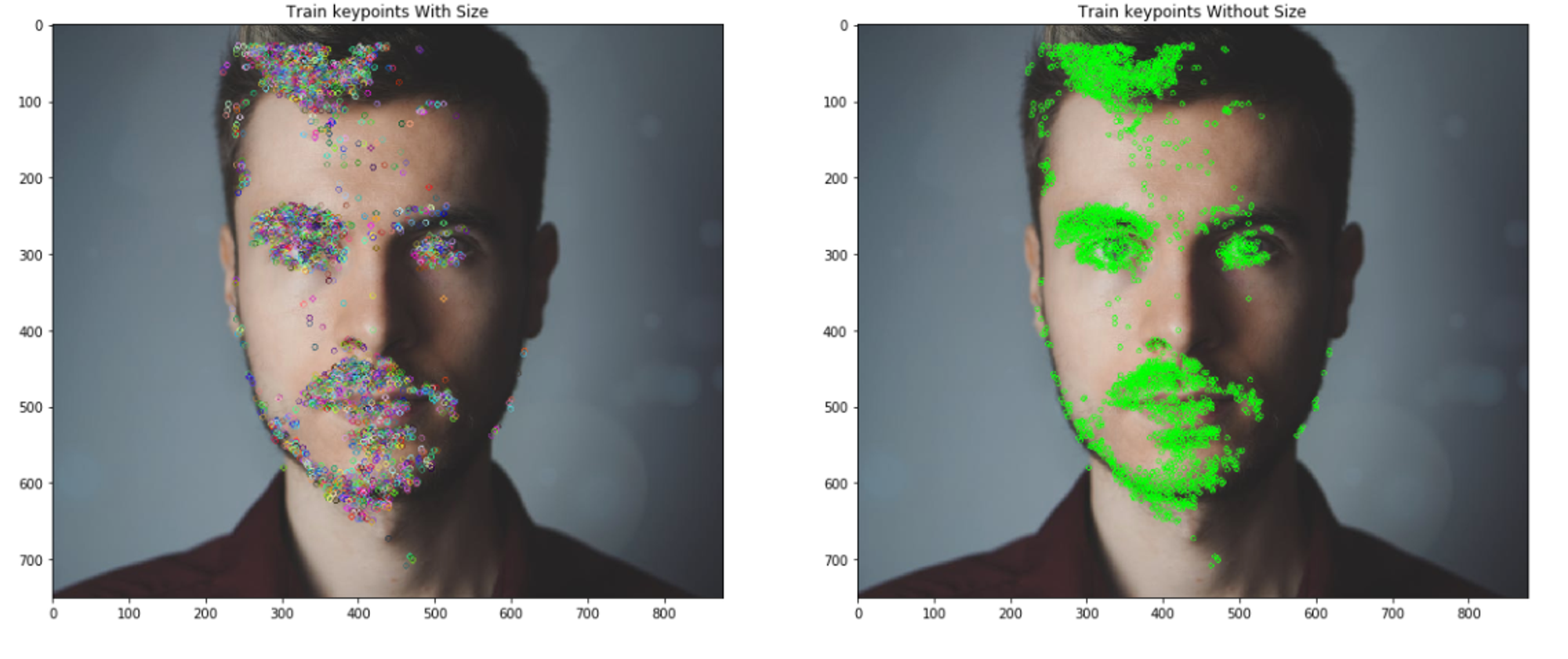
keypoints_without_size = np.copy(training_image)
keypoints_with_size = np.copy(training_image)

cv2.drawKeypoints(training_image, train_keypoints, keypoints_without_size, color = (0, 255, 0))

cv2.drawKeypoints(training_image, train_keypoints, keypoints_with_size, flags = cv2.DRAW_MATCHES_FLAGS_DRAW_RICH_KEYPOINTS)

Python

Copy

# Create a Brute Force Matcher object.
bf = cv2.BFMatcher(cv2.NORM_HAMMING, crossCheck = True)
# Perform the matching between the BRIEF descriptors of the training image and the test image
matches = bf.match(train_descriptor, test_descriptor)
# The matches with shorter distance are the ones we want.
matches = sorted(matches, key = lambda x : x.distance)

result = cv2.drawMatches(training_image, train_keypoints, test_gray, test_keypoints, matches, test_gray, flags = 2)

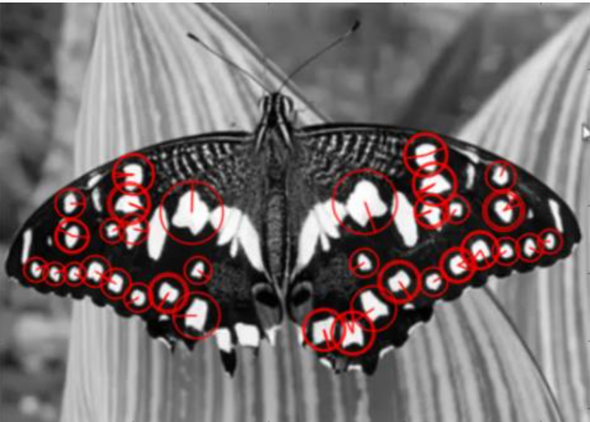
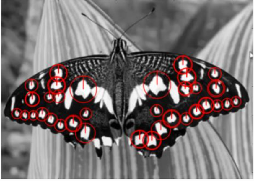
Oriented FAST and rotated BRIEF (ORB)

https://medium.com/data-breach/introduction-to-orb-oriented-fast-and-rotated-brief-4220e8ec40cf

https://docs.opencv.org/3.4/dc/d16/tutorial_akaze_tracking.html

https://opencv24-python-tutorials.readthedocs.io/en/latest/py_tutorials/py_feature2d/py_orb/py_orb.html#orb

Beyond FAST

Given a pixel p in an array fast compares the brightness of p to surrounding 16 pixels that are in a small circle around p. 

Pixels in the circle is then sorted into three classes (lighter than p, darker than p or similar to p). If more than 8 pixels are darker or brighter than p than it is selected as a keypoint

However, FAST features do not have an orientation component and multiscale features

ORB is partial scale invariant, by detecting keypoints at each level of the multiscale image pyramid

We oriente keypoints by considering O (center of the corner) and C (centroid of the corner)

Moments of the patch: ∑x,yxpyqI(x,y)\sum_{x,y}x^py^qI(x,y)∑x,y​xpyqI(x,y)﻿​

Centroid: C=(m10m00,m01m00)C=(\frac{m_{10}}{m_{00}},\frac{m_{01}}{m_{00}})C=(m00​m10​​,m00​m01​​)﻿, and orientation θ=atan2(m01,m10)\theta=atan2(m_{01},m_{10})θ=atan2(m01​,m10​)﻿​

We can rotate patch to a canonical orientation to get descriptor, achieving rotational invariance

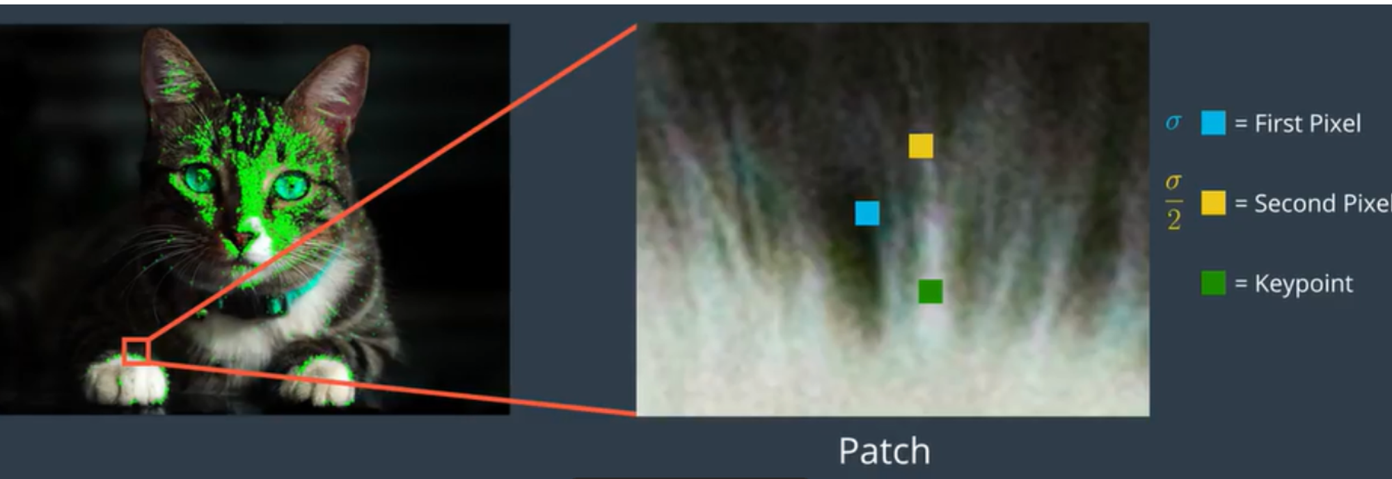
Beyond BRIEF

Brief takes all keypoints found by the FAST algorithm and convert it into a binary feature vector so that together they can represent an object

Here we choose 128 pairs from a keypoint by sampling a Gaussian distribution around it, and then sampling the second pixel around the first pixel with a Gaussian distribution of scale σ/2\sigma/2σ/2﻿​

However BRIEF is not invariant to rotation, so we use Rotation-aware BRIEF (rBRIEF), so ORB propose a method to steer BRIEF according to keypoints orientation

For nnn﻿ binary test at (xi,yi)(x_i,y_i)(xi​,yi​)﻿ the set of points is S=[x1...xny1...yn]S=\begin{bmatrix} x_1 & ... &x_n
\\ y_1 &...&y_n \end{bmatrix}S=[x1​y1​​......​xn​yn​​]﻿​

Using the patch orientation θ\thetaθ﻿, the rotation matrix is Rθ=[cos(θ)−sin(θ)sin(θ)cos(θ)]R_{\theta}=\begin{bmatrix}cos(\theta) &-sin(\theta) \\sin(\theta) & cos(\theta)\end{bmatrix}Rθ​=[cos(θ)sin(θ)​−sin(θ)cos(θ)​]﻿​

Sθ=RθSS_{\theta}=R_{\theta}SSθ​=Rθ​S﻿​

ORB discretize the angle to increments of (12 degrees), and construct a lookup table of precomputed BRIEF patterns

Greedy search among all possible binary tests to find the ones that have both high variance and means close to 0.5, as well as being uncorrelated. The result is called rBRIEF.

Shell

Copy

# Initiate STAR detector
orb = cv2.ORB()
# find the keypoints with ORB
kp = orb.detect(img,None)
# compute the descriptors with ORB
kp, des = orb.compute(img, kp)
# draw only keypoints location,not size and orientation
img2 = cv2.drawKeypoints(img,kp,color=(0,255,0), flags=0)
plt.imshow(img2),plt.show()

Feature Matcher

https://docs.opencv.org/3.4/d5/d6f/tutorial_feature_flann_matcher.html

https://opencv24-python-tutorials.readthedocs.io/en/latest/py_tutorials/py_feature2d/py_matcher/py_matcher.html#matcher

Classical feature descriptors (SIFT, SURF) are usually compared and matched using the Euclidean distance (or L2-norm). 

Since SIFT and SURF descriptors represent the histogram of oriented gradient (of the Haar wavelet response for SURF) in a neighborhood, alternatives of the Euclidean distance are histogram-based metrics ( χ2, Earth Mover’s Distance (EMD), ...).

Binary descriptors (ORB, BRIEF, BRISK) are matched using the Hamming distance. This distance is equivalent to count the number of different elements for binary strings (population count after applying a XOR operation):

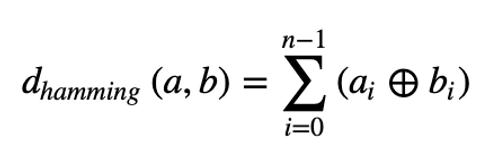
To filter the matches, use a distance ratio test to try to eliminate false matches. 

The distance ratio between the two nearest matches of a considered keypoint is computed and it is a good match when this value is below a threshold. 

This ratio allows helping to discriminate between ambiguous matches (distance ratio between the two nearest neighbors is close to one) and well discriminated matches.

Brute force

cv2.BFMatcher() takes 2 args

normType: use cv2.NORM_L2 for SIFT or SURF and use cv2.NORM_HAMMING for binary string descriptor (BRIEF, BRISK, ORB)

crosscheck False by default. If True, matcher ensure that 2 features in 2 different sets match each other. Consistent results, and good alternative to ratio test.

Then we can either

matcher.match() : best match

matcher.knnMatch(): k best matches

Shell

Copy

orb = cv2.ORB()
# find the keypoints and descriptors with ORB
kp1, des1 = orb.detectAndCompute(img1, None)
kp2, des2 = orb.detectAndCompute(img2, None)
# create BFMatcher object
bf = cv2.BFMatcher(cv2.NORM_HAMMING, crossCheck=True)
# Match descriptors.
matches = bf.match(des1,des2)
# Sort them in the order of their distance.
matches = sorted(matches, key=lambda x:x.distance)
# Draw first 10 matches.
img3 = cv2.drawMatches(img1,kp1,img2,kp2,matches[:10], flags=2)

plt.imshow(img3)
plt.show()

Fast Library for Approximate Nearest Neighbors (FLANN)

2 parameters

IndexParams

For SIFT, SURF:

Python

Copy

 index_params = dict(
		algorithm=FLANN_INDEX_KDTREE,
		trees=5,
)

For ORB: 

Python

Copy

index_params= dict(
		algorithm=FLANN_INDEX_LSH,
    table_number=6, # 12
    key_size=12, # 20
    multi_probe_level=1 # 2
)

SearchParams: specifies the number of times the trees in the index should be recursively traversed.

Python

Copy

search_params = dict(checks=100)

Implementation

Python

Copy

sift = cv2.SIFT()
# find the keypoints and descriptors with SIFT
kp1, des1 = sift.detectAndCompute(img1,None)
kp2, des2 = sift.detectAndCompute(img2,None)
# FLANN parameters
FLANN_INDEX_KDTREE = 0
index_params = dict(algorithm = FLANN_INDEX_KDTREE, trees = 5)
search_params = dict(checks=50) # or pass empty dictionary

flann = cv2.FlannBasedMatcher(index_params,search_params)

matches = flann.knnMatch(des1,des2,k=2)
# Need to draw only good matches, so create a mask
matchesMask = [[0,0] for i in xrange(len(matches))]
# ratio test as per Lowe's paper
for i,(m,n) in enumerate(matches):
if m.distance < 0.7*n.distance:
        matchesMask[i]=[1,0]

draw_params = dict(matchColor = (0,255,0),
                   singlePointColor = (255,0,0),
                   matchesMask = matchesMask,
                   flags = 0)

img3 = cv2.drawMatchesKnn(img1,kp1,img2,kp2,matches,None,**draw_params)

plt.imshow(img3,)
plt.show()

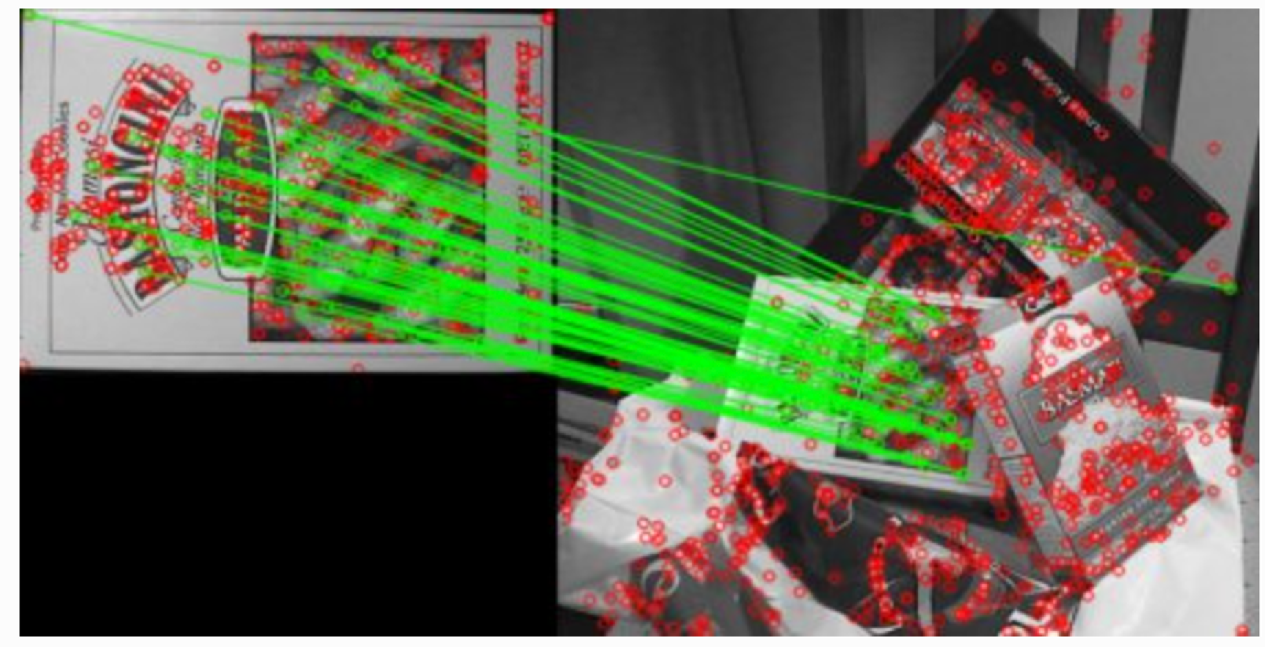
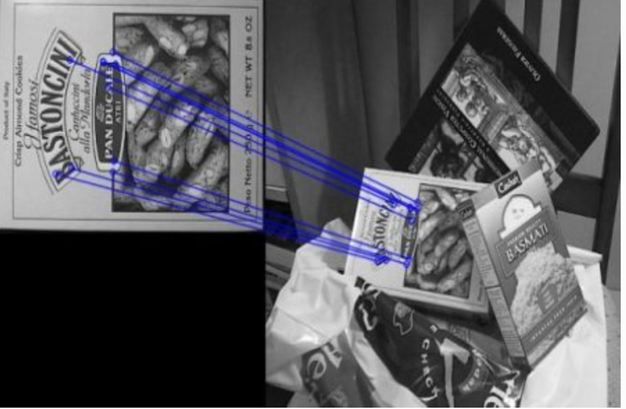
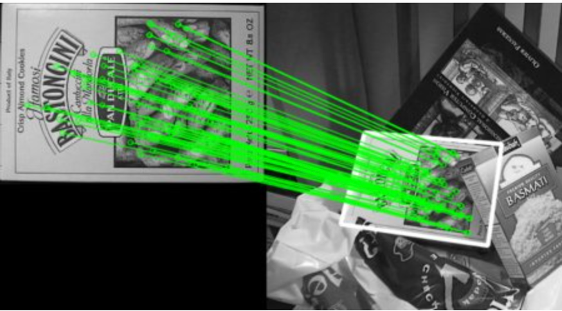
Homography

https://opencv24-python-tutorials.readthedocs.io/en/latest/py_tutorials/py_feature2d/py_feature_homography/py_feature_homography.html#feature-homography

https://docs.opencv.org/3.4/d9/dab/tutorial_homography.html

If enough matches are found, we extract the locations of matched keypoints in both the images.

They are passed to findHomography to find the perpective transformation. 

Once we get this 3x3 transformation matrix M, we use perspectiveTransform to transform the corners of queryImage to corresponding points in trainImage.

Python

Copy

import numpy as np
import cv2
from matplotlib import pyplot as plt

MIN_MATCH_COUNT = 10

img1 = cv2.imread('box.png',0) # queryImage
img2 = cv2.imread('box_in_scene.png',0) # trainImage
# Initiate SIFT detector
sift = cv2.SIFT()
# find the keypoints and descriptors with SIFT
kp1, des1 = sift.detectAndCompute(img1,None)
kp2, des2 = sift.detectAndCompute(img2,None)

FLANN_INDEX_KDTREE = 0
index_params = dict(algorithm = FLANN_INDEX_KDTREE, trees = 5)
search_params = dict(checks = 50)

flann = cv2.FlannBasedMatcher(index_params, search_params)

matches = flann.knnMatch(des1,des2,k=2)
# store all the good matches as per Lowe's ratio test.
good = []
for m,n in matches:
if m.distance < 0.7*n.distance:
        good.append(m)
if len(good)>MIN_MATCH_COUNT:
    src_pts = np.float32([ kp1[m.queryIdx].pt for m in good ]).reshape(-1,1,2)
    dst_pts = np.float32([ kp2[m.trainIdx].pt for m in good ]).reshape(-1,1,2)

    M, mask = cv2.findHomography(src_pts, dst_pts, cv2.RANSAC,5.0)
    matchesMask = mask.ravel().tolist()

    h,w = img1.shape
    pts = np.float32([ [0,0],[0,h-1],[w-1,h-1],[w-1,0] ]).reshape(-1,1,2)
    dst = cv2.perspectiveTransform(pts,M)

    img2 = cv2.polylines(img2,[np.int32(dst)],True,255,3, cv2.LINE_AA)
else:
print "Not enough matches are found - %d/%d" % (len(good),MIN_MATCH_COUNT)
    matchesMask = None

draw_params = dict(matchColor = (0,255,0), # draw matches in green color
                   singlePointColor = None,
                   matchesMask = matchesMask, # draw only inliers
                   flags = 2)

img3 = cv2.drawMatches(img1,kp1,img2,kp2,good,None,**draw_params)

plt.imshow(img3, 'gray'),plt.show()

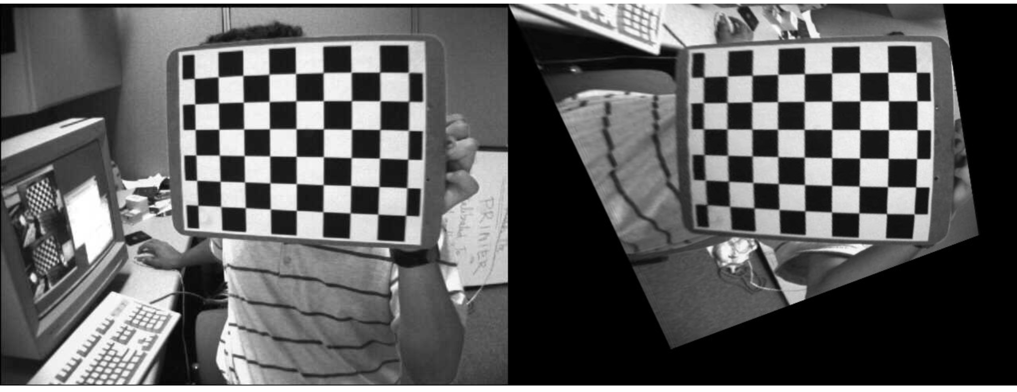
Perspective correction

Python

Copy

ret1, corners1 = cv.findChessboardCorners(img1, patternSize)
ret2, corners2 = cv.findChessboardCorners(img2, patternSize)

H, _ = cv.findHomography(corners1, corners2)
print(H)

img1_warp = cv.warpPerspective(img1, H, (img1.shape[1], img1.shape[0]))

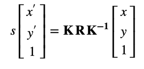
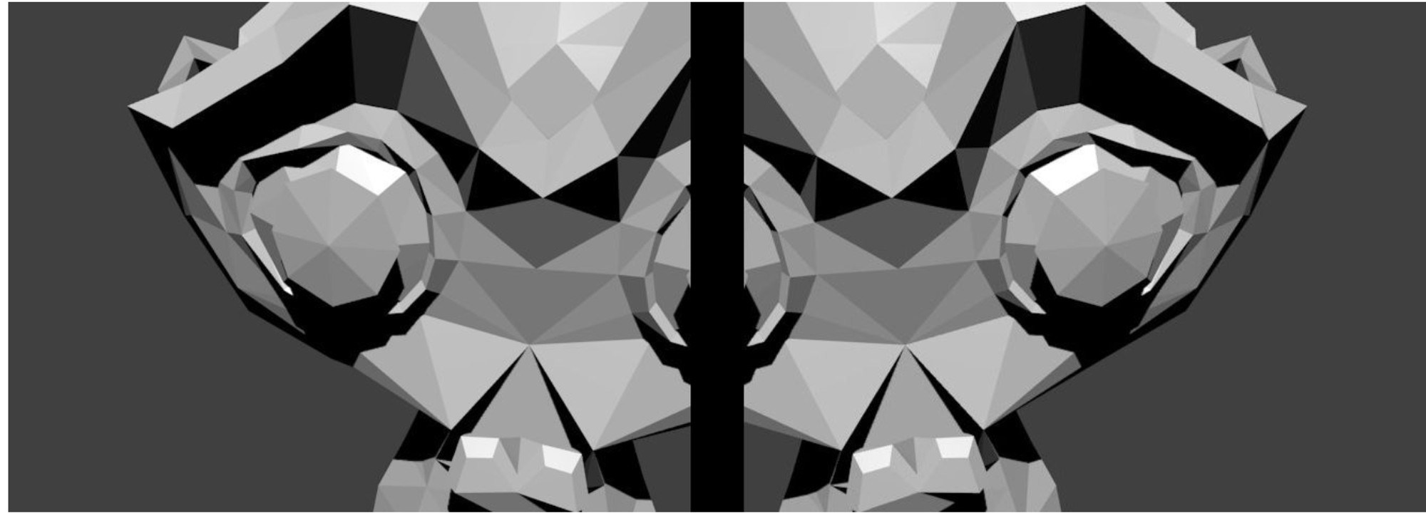
Panorama stitching

The homography transformation applies only for planar structure. 

But in the case of a rotating camera (pure rotation around the camera axis of projection, no translation), an arbitrary world can be considered

The homography can then be computed using the rotation transformation and the camera intrinsic parameters

Python

Copy

R1 = c1Mo[0:3, 0:3]
R2 = c2Mo[0:3, 0:3]

R2 = R2.transpose()
R_2to1 = np.dot(R1,R2)

H = cameraMatrix.dot(R_2to1).dot(np.linalg.inv(cameraMatrix))
H = H / H[2][2]

img_stitch = cv.warpPerspective(img2, H, (img2.shape[1]*2, img2.shape[0]))
img_stitch[0:img1.shape[0], 0:img1.shape[1]] = img1