Background Substraction (BS)
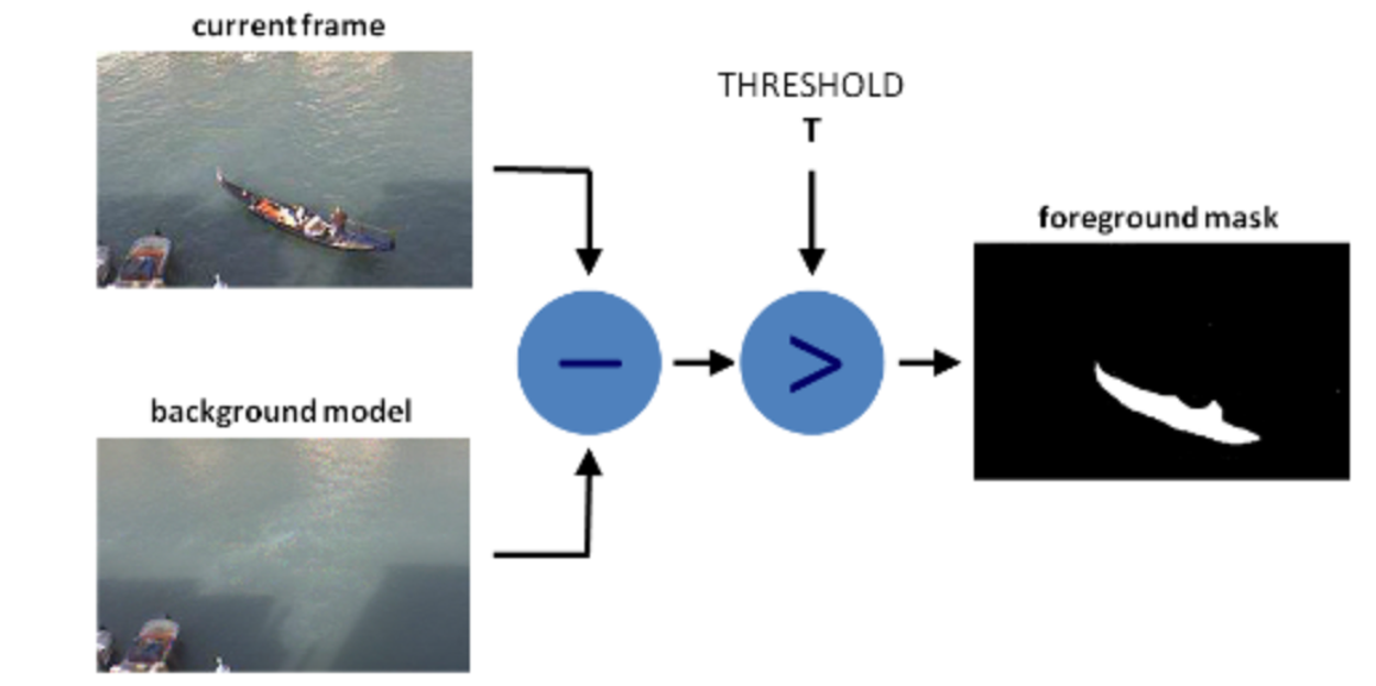
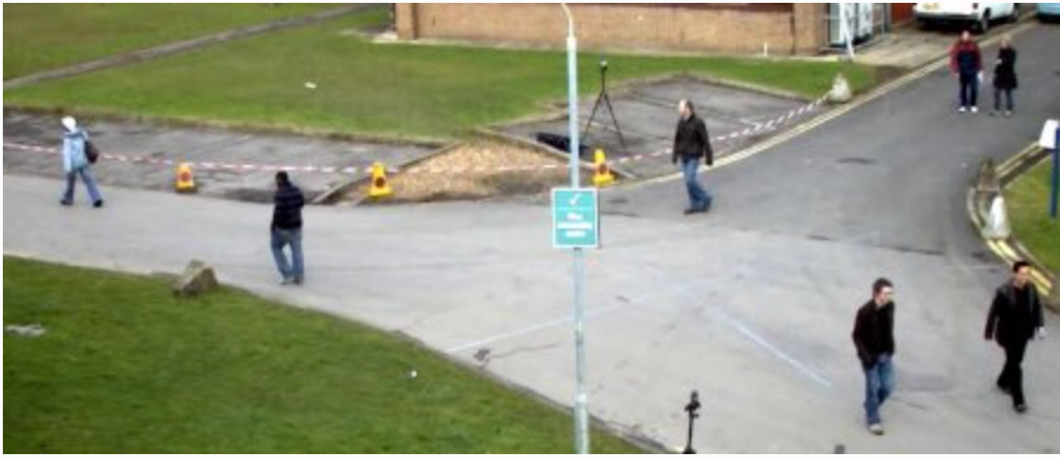
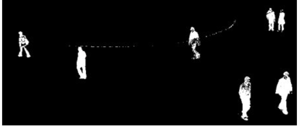
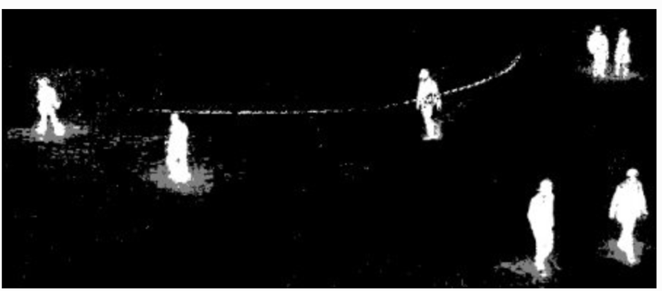
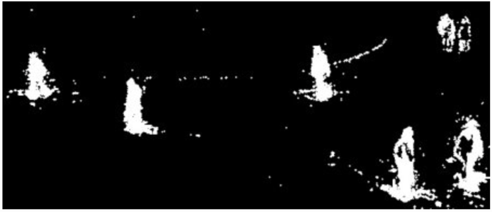
Goal is generating a foreground mask (a binary image containing the pixels belonging to moving objects in the scene) by using static cameras.
BS calculates the foreground mask performing a subtraction between the current frame and a background model, containing the static part of the scene
Back ground modeling is made of 2 steps:
Background initialization
Back ground update, to adapt to possible changes
But in most of the cases, you may not have a image without people or cars to init, so we need to extract the background from whatever images we have.
It become more complicated when there is shadow of the vehicles. Since shadow is also moving, simple subtraction will mark that also as foreground. It complicates things.
BackGroundSubstractorMOG
Gaussian Mixture-based Background/Foreground Segmentation Algorithm.
Model each background pixel by a mixture of K Gaussian distributions (K = 3 to 5).
The weights of the mixture represent the time proportions that those colours stay in the scene.
The probable background colours are the ones which stay longer and more static.
BackGroundSubstractorMOG2
BackgroundSubtractorGMG
full script
Python
Copy
from __future__ import print_function
import cv2 as cv
import argparse
parser = argparse.ArgumentParser(description='This program shows how to use background subtraction methods provided by \
OpenCV. You can process both videos and images.')
parser.add_argument('--input', type=str, help='Path to a video or a sequence of image.', default='vtest.avi')
parser.add_argument('--algo', type=str, help='Background subtraction method (KNN, MOG2).', default='MOG2')
args = parser.parse_args()
if args.algo == 'MOG2':
backSub = cv.createBackgroundSubtractorMOG2()
else:
backSub = cv.createBackgroundSubtractorKNN()
#capture = cv.VideoCapture(cv.samples.findFileOrKeep(args.input))
capture = cv.VideoCapture(0)
if not capture.isOpened:
print('Unable to open: ' + args.input)
exit(0)
while True:
ret, frame = capture.read()
if frame is None:
break
fgMask = backSub.apply(frame)
cv.rectangle(frame, (10, 2), (100,20), (255,255,255), -1)
cv.putText(frame, str(capture.get(cv.CAP_PROP_POS_FRAMES)), (15, 15),
cv.FONT_HERSHEY_SIMPLEX, 0.5 , (0,0,0))
cv.imshow('Frame', frame)
cv.imshow('FG Mask', fgMask)
keyboard = cv.waitKey(30)
if keyboard == 'q' or keyboard == 27:
break
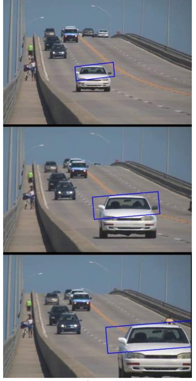
Mean Shift and CamShift
Meanshift
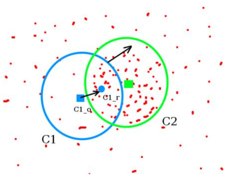
Start by computing back projection using a ROI window
Computing difference between circle windows center and points centroid, update the center with the centroid, until convergence
So finally what you obtain is a window with maximum pixel distribution.
Continuously Adaptive Meanshift: Camshift
The issue with meanshift is that our window has always the same size
Applies meanshift first.
Once meanshift converges, update the window size as
Also compute the orientation of the best fitting ellipse
Implementation
Python
Copy
import numpy as np
import cv2
cap = cv2.VideoCapture('slow.flv')
# take first frame of the video
ret,frame = cap.read()
# setup initial location of window
r,h,c,w = 250,90,400,125 # simply hardcoded the values
track_window = (c,r,w,h)
# set up the ROI for tracking
roi = frame[r:r+h, c:c+w]
hsv_roi = cv2.cvtColor(frame, cv2.COLOR_BGR2HSV)
mask = cv2.inRange(hsv_roi, np.array((0., 60.,32.)), np.array((180.,255.,255.)))
roi_hist = cv2.calcHist([hsv_roi],[0],mask,[180],[0,180])
cv2.normalize(roi_hist,roi_hist,0,255,cv2.NORM_MINMAX)
# Setup the termination criteria, either 10 iteration or move by atleast 1 pt
term_crit = ( cv2.TERM_CRITERIA_EPS | cv2.TERM_CRITERIA_COUNT, 10, 1 )
while(1):
ret ,frame = cap.read()
if ret == True:
hsv = cv2.cvtColor(frame, cv2.COLOR_BGR2HSV)
dst = cv2.calcBackProject([hsv],[0],roi_hist,[0,180],1)
# apply meanshift to get the new location
ret, track_window = cv2.CamShift(dst, track_window, term_crit)
# Draw it on image
pts = cv2.boxPoints(ret)
pts = np.int0(pts)
img2 = cv2.polylines(frame,[pts],True, 255,2)
cv2.imshow('img2',img2)
k = cv2.waitKey(60) & 0xff
if k == 27:
break
else:
cv2.imwrite(chr(k)+".jpg",img2)
else:
break
cv2.destroyAllWindows()
cap.release()
hardcode initial track_window
inRange on initial ROI to filter low saturation and low visibility
track_window computed iteratively and passed as a argument
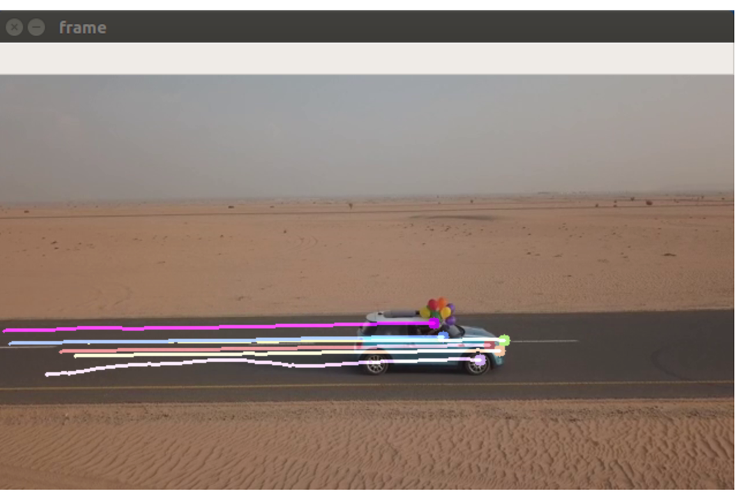
Optical Flow
Sparse
Hypothesis
The pixel intensities of an object do not change between consecutive frames.
Neighbouring pixels have similar motion.
Optical flow equation
using Taylor
,
with , , ,
are unknown. We solve it using Lucas-Kanade
Kanade:
Takes a 3x3 patch around the point. So all the 9 points have the same motion
We can find for these 9 points, ie solving 9 equations with two unknown variables, which is over-determined
ie
Least squares
thus
Fails when there is a large motion
To deal with this we use pyramids: multi-scaling trick.
When we go up in the pyramid, small motions are removed and large motions become small motions.
We find corners in the image using Shi-Tomasi corner detector and then calculate the corners’ motion vector between two consecutive frames.
full script
Python
Copy
# params for ShiTomasi corner detection
feature_params = dict( maxCorners = 100,
qualityLevel = 0.3,
minDistance = 7,
blockSize = 7 )
# Parameters for lucas kanade optical flow
lk_params = dict( winSize = (15,15),
maxLevel = 2,
criteria = (cv.TERM_CRITERIA_EPS | cv.TERM_CRITERIA_COUNT, 10, 0.03))
# Create some random colors
color = np.random.randint(0,255,(100,3))
# Take first frame and find corners in it
ret, old_frame = cap.read()
old_gray = cv.cvtColor(old_frame, cv.COLOR_BGR2GRAY)
p0 = cv.goodFeaturesToTrack(old_gray, mask = None, **feature_params)
# Create a mask image for drawing purposes
mask = np.zeros_like(old_frame)
while(1):
ret,frame = cap.read()
frame_gray = cv.cvtColor(frame, cv.COLOR_BGR2GRAY)
# calculate optical flow
p1, st, err = cv.calcOpticalFlowPyrLK(old_gray, frame_gray, p0, None, **lk_params)
# Select good points
good_new = p1[st==1]
good_old = p0[st==1]
# draw the tracks
for i,(new,old) in enumerate(zip(good_new, good_old)):
a,b = new.ravel()
c,d = old.ravel()
mask = cv.line(mask, (a,b),(c,d), color[i].tolist(), 2)
frame = cv.circle(frame,(a,b),5,color[i].tolist(),-1)
img = cv.add(frame ,mask)
cv.imshow('frame', img)
k = cv.waitKey(30) & 0xff
if k == 27:
break
# Now update the previous frame and previous points
old_gray = frame_gray.copy()
p0 = good_new.reshape(-1,1,2)
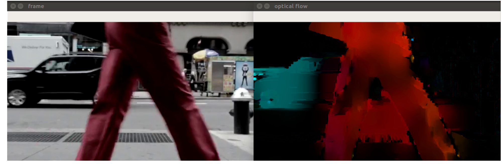
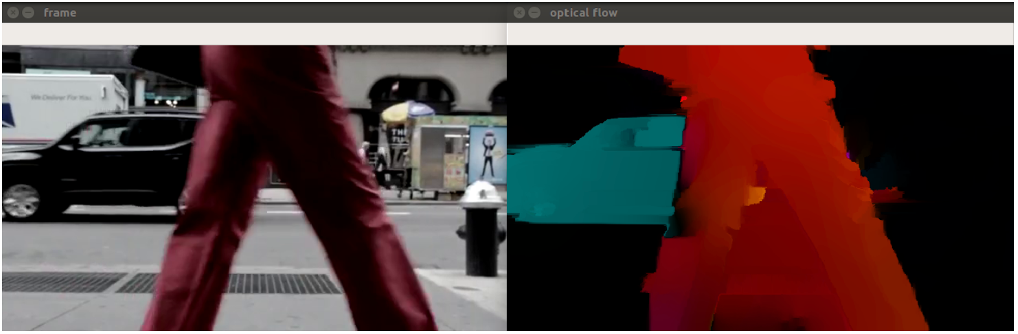
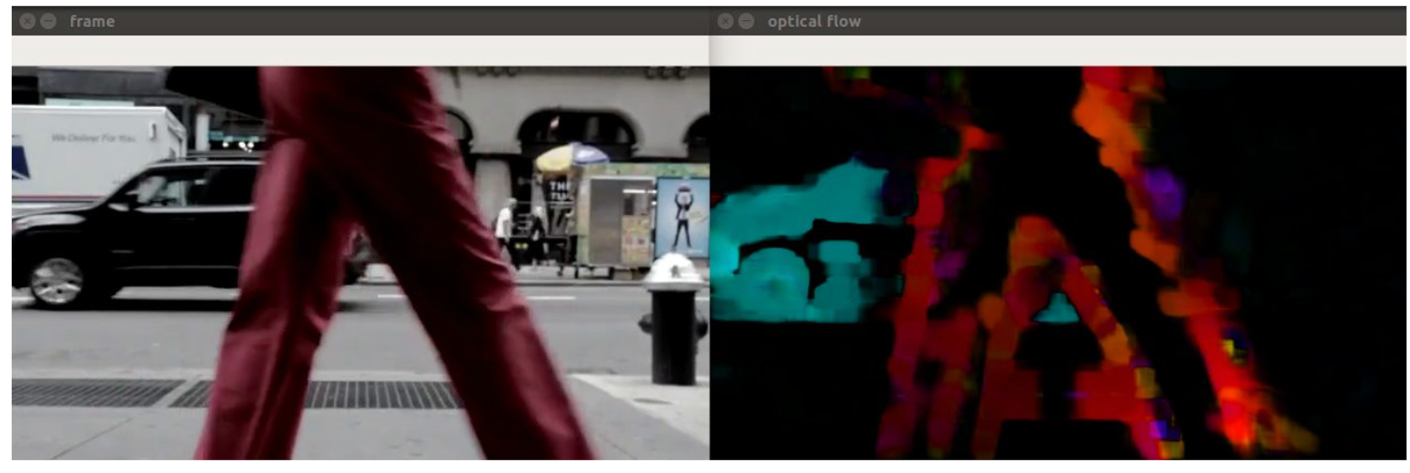
Dense
Compute motion for every pixel in the image
Python
Copy
def dense_optical_flow(method, video_path, params=[], to_gray=False):
# Read the video and first frame
cap = cv2.VideoCapture(video_path)
ret, old_frame = cap.read()
# crate HSV & make Value a constant
hsv = np.zeros_like(old_frame)
hsv[..., 1] = 255
# Preprocessing for exact method
if to_gray:
old_frame = cv2.cvtColor(old_frame, cv2.COLOR_BGR2GRAY)
while True:
# Read the next frame
ret, new_frame = cap.read()
frame_copy = new_frame
if not ret:
break
# Preprocessing for exact method
if to_gray:
new_frame = cv2.cvtColor(new_frame, cv2.COLOR_BGR2GRAY)
# Calculate Optical Flow
flow = method(old_frame, new_frame, None, *params)
# Encoding: convert the algorithm's output into Polar coordinates
mag, ang = cv2.cartToPolar(flow[..., 0], flow[..., 1])
# Use Hue and Value to encode the Optical Flow
hsv[..., 0] = ang * 180 / np.pi / 2
hsv[..., 2] = cv2.normalize(mag, None, 0, 255, cv2.NORM_MINMAX)
# Convert HSV image into BGR for demo
bgr = cv2.cvtColor(hsv, cv2.COLOR_HSV2BGR)
cv2.imshow("frame", frame_copy)
cv2.imshow("optical flow", bgr)
k = cv2.waitKey(25) & 0xFF
if k == 27:
break
# Update the previous frame
old_frame = new_frame
Dense Pyramid Lucas-Kanade algorithm
Python
Copy
elif args.algorithm == 'lucaskanade_dense':
method = cv2.optflow.calcOpticalFlowSparseToDense
frames = dense_optical_flow(method, video_path, save, to_gray=True)
Farneback algorithm
Approximate some neighbors of each pixel with a polynomial, taking the second order of Taylor expansion
We observe the differences in the approximated polynomials caused by object displacements
Python
Copy
elif args.algorithm == 'farneback':
method = cv2.calcOpticalFlowFarneback
params = [0.5, 3, 15, 3, 5, 1.2, 0] # default Farneback's algorithm parameters
frames = dense_optical_flow(method, video_path, save, params, to_gray=True)
RLOF
The intensity constancy assumption doesn’t fully reflect how the real world behaves.
There are also shadows, reflections, weather conditions, moving light sources, and, in short, varying illuminations.
with illumination parameters
Python
Copy
elif args.algorithm == "rlof":
method = cv2.optflow.calcOpticalFlowDenseRLOF
frames = dense_optical_flow(method, video_path, save)