Video Analysis

https://docs.opencv.org/4.5.0/da/dd0/tutorial_table_of_content_video.html (opens in a new tab)

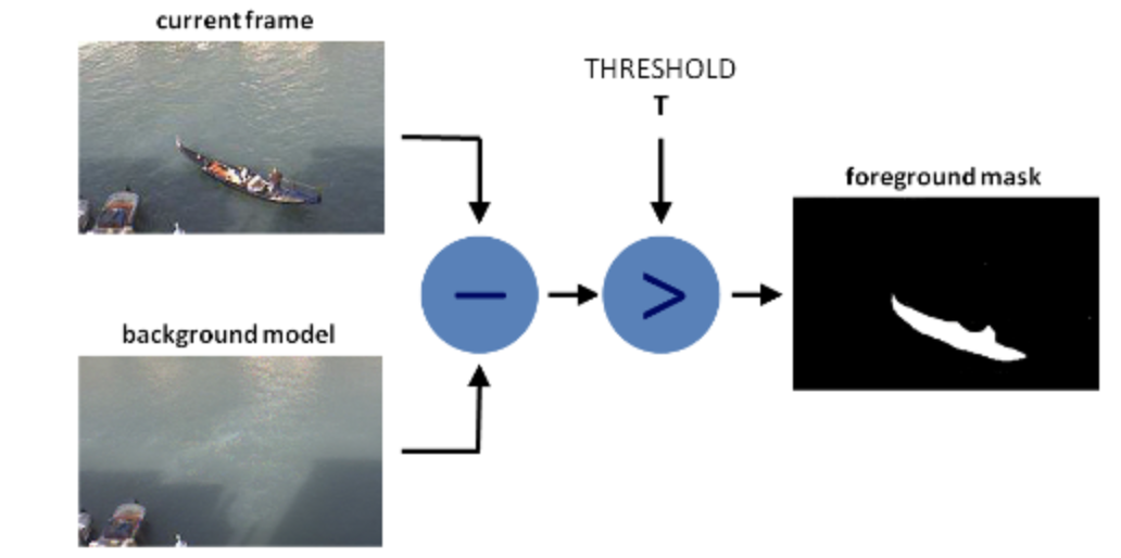
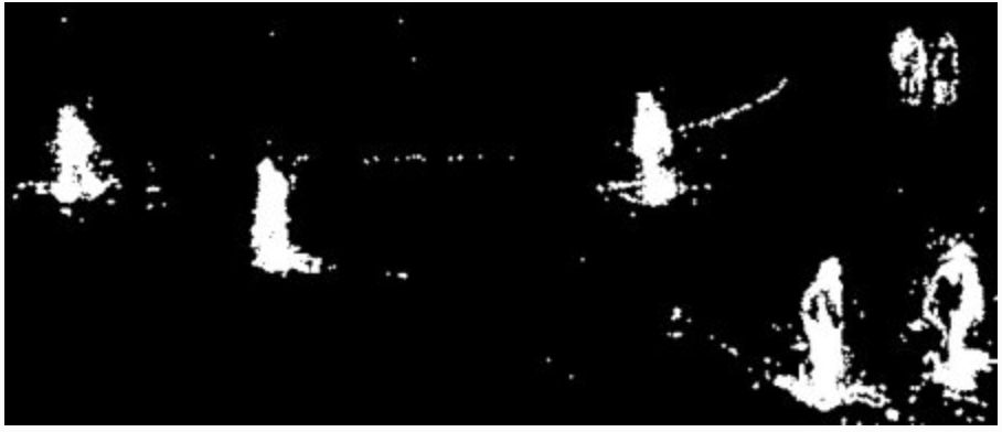
Background Substraction (BS)

Goal is generating a foreground mask (a binary image containing the pixels belonging to moving objects in the scene) by using static cameras.
BS calculates the foreground mask performing a subtraction between the current frame and a background model, containing the static part of the scene

Screen Shot 2021-12-03 at 11.16.37.png

Back ground modeling is made of 2 steps:
1. Background initialization
2. Back ground update, to adapt to possible changes
But in most of the cases, you may not have a image without people or cars to init, so we need to extract the background from whatever images we have.
It become more complicated when there is shadow of the vehicles. Since shadow is also moving, simple subtraction will mark that also as foreground. It complicates things.

Screen Shot 2021-12-03 at 11.50.49.png

BackGroundSubstractorMOG
- Gaussian Mixture-based Background/Foreground Segmentation Algorithm.
- Model each background pixel by a mixture of K Gaussian distributions (K = 3 to 5).
- The weights of the mixture represent the time proportions that those colours stay in the scene.
- The probable background colours are the ones which stay longer and more static.
BackGroundSubstractorMOG2
BackgroundSubtractorGMG

full script

from __future__ import print_function
import cv2 as cv
import argparse
 
parser = argparse.ArgumentParser(description='This program shows how to use background subtraction methods provided by \
                                              OpenCV. You can process both videos and images.')
parser.add_argument('--input', type=str, help='Path to a video or a sequence of image.', default='vtest.avi')
parser.add_argument('--algo', type=str, help='Background subtraction method (KNN, MOG2).', default='MOG2')
 
args = parser.parse_args()
if args.algo == 'MOG2':
    backSub = cv.createBackgroundSubtractorMOG2()
else:
    backSub = cv.createBackgroundSubtractorKNN()
 
#capture = cv.VideoCapture(cv.samples.findFileOrKeep(args.input))
capture = cv.VideoCapture(0)
if not capture.isOpened:
    print('Unable to open: ' + args.input)
    exit(0)
 
while True:
    ret, frame = capture.read()
    if frame is None:
        break
    
    fgMask = backSub.apply(frame)
    
    cv.rectangle(frame, (10, 2), (100,20), (255,255,255), -1)
    cv.putText(frame, str(capture.get(cv.CAP_PROP_POS_FRAMES)), (15, 15),
               cv.FONT_HERSHEY_SIMPLEX, 0.5 , (0,0,0))
    
    cv.imshow('Frame', frame)
    cv.imshow('FG Mask', fgMask)
    
    keyboard = cv.waitKey(30)
    if keyboard == 'q' or keyboard == 27:
        break

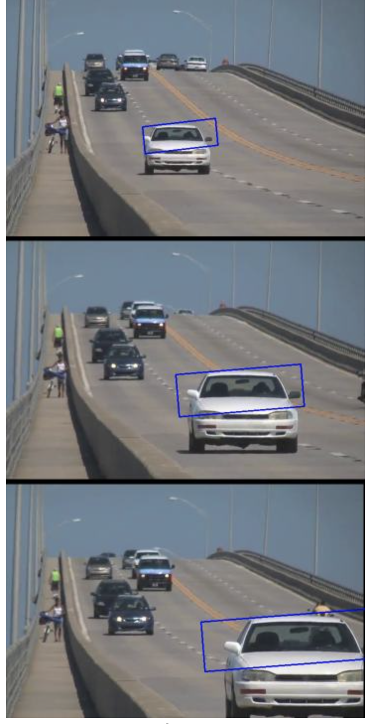
Mean Shift and CamShift

https://opencv24-python-tutorials.readthedocs.io/en/latest/py_tutorials/py_video/py_meanshift/py_meanshift.html#meanshift (opens in a new tab)

Meanshift
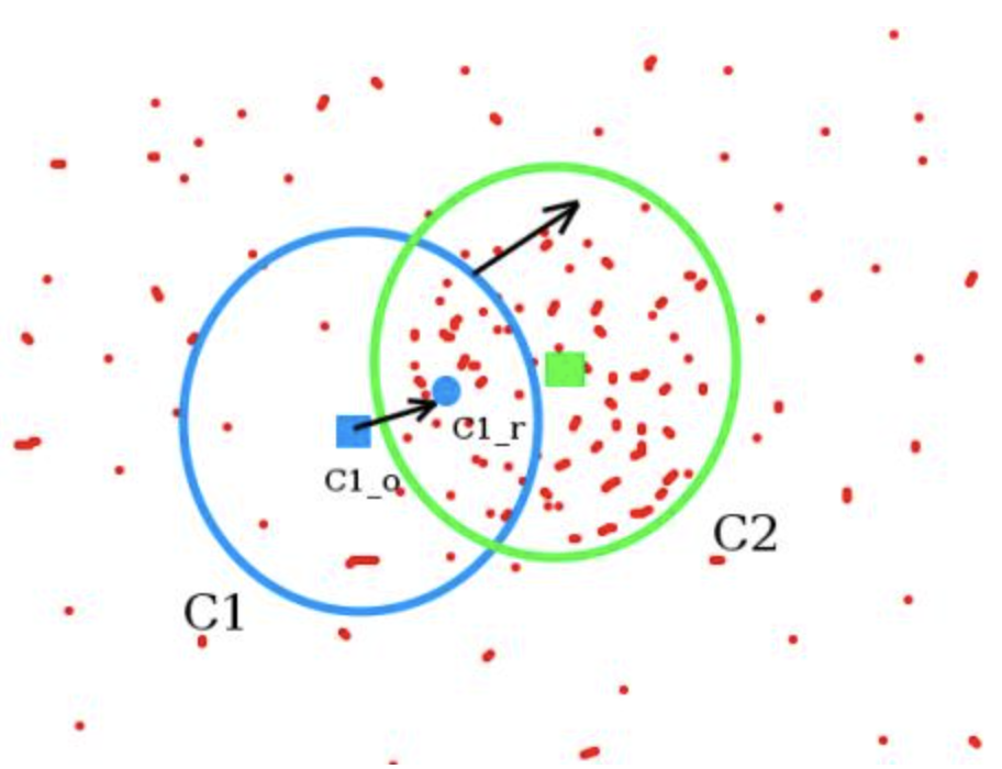
- Start by computing back projection using a ROI window
- Computing difference between circle windows center and points centroid, update the center with the centroid, until convergence
- So finally what you obtain is a window with maximum pixel distribution.

Continuously Adaptive Meanshift: Camshift

The issue with meanshift is that our window has always the same size
Applies meanshift first.
Once meanshift converges, update the window size as $s=2\sqrt{\frac{M_{00}}{256}}$
Also compute the orientation of the best fitting ellipse

Implementation

import numpy as np
import cv2
 
cap = cv2.VideoCapture('slow.flv')
 
# take first frame of the video
ret,frame = cap.read()
 
# setup initial location of window
r,h,c,w = 250,90,400,125  # simply hardcoded the values
track_window = (c,r,w,h)
 
# set up the ROI for tracking
roi = frame[r:r+h, c:c+w]
hsv_roi =  cv2.cvtColor(frame, cv2.COLOR_BGR2HSV)
mask = cv2.inRange(hsv_roi, np.array((0., 60.,32.)), np.array((180.,255.,255.)))
roi_hist = cv2.calcHist([hsv_roi],[0],mask,[180],[0,180])
cv2.normalize(roi_hist,roi_hist,0,255,cv2.NORM_MINMAX)
 
# Setup the termination criteria, either 10 iteration or move by atleast 1 pt
term_crit = ( cv2.TERM_CRITERIA_EPS | cv2.TERM_CRITERIA_COUNT, 10, 1 )
 
while(1):
    ret ,frame = cap.read()
 
    if ret == True:
        hsv = cv2.cvtColor(frame, cv2.COLOR_BGR2HSV)
        dst = cv2.calcBackProject([hsv],[0],roi_hist,[0,180],1)
 
        # apply meanshift to get the new location
        ret, track_window = cv2.CamShift(dst, track_window, term_crit)
 
        # Draw it on image
        pts = cv2.boxPoints(ret)
        pts = np.int0(pts)
        img2 = cv2.polylines(frame,[pts],True, 255,2)
        cv2.imshow('img2',img2)
 
        k = cv2.waitKey(60) & 0xff
        if k == 27:
            break
        else:
            cv2.imwrite(chr(k)+".jpg",img2)
 
    else:
        break
 
cv2.destroyAllWindows()
cap.release()

hardcode initial track_window
inRange on initial ROI to filter low saturation and low visibility
track_window computed iteratively and passed as a argument

Screen Shot 2021-12-07 at 08.28.23.png

Optical Flow

https://docs.opencv.org/4.5.0/d4/dee/tutorial_optical_flow.html (opens in a new tab)

https://learnopencv.com/optical-flow-in-opencv/ (opens in a new tab)

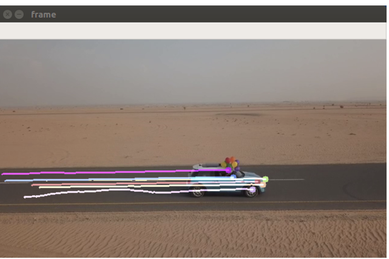
Sparse

Screen Shot 2021-12-08 at 09.06.40.png

Hypothesis
1. The pixel intensities of an object do not change between consecutive frames.
2. Neighbouring pixels have similar motion.
Optical flow equation

$I(x,y,t)=I(x+dx,y+dy,t+dt)$

using Taylor

$uf_x+vf_y+f_t=0$ ,

with $f_x=\frac{\partial I}{\partial x}$ , $f_y=\frac{\partial I}{\partial y}$ , $u=\frac{dx}{dt}$ , $v=\frac{dy}{dt}$

$u, v$ are unknown. We solve it using Lucas-Kanade
Kanade:
- Takes a 3x3 patch around the point. So all the 9 points have the same motion
- We can find $(f_x,f_y,f_t)$ for these 9 points, ie solving 9 equations with two unknown variables, which is over-determined
- $f_x(p_1)u+f_y(p_1)v=-f_t(p_1)\\ ... \\ f_x(p_9)v+f_y(p_9)v=-f_t(p_9)$
  
  ie
  
  $\begin{bmatrix} f_x(p_1) & f_y(p_1) \\ ... & ...\\ f_x(p_9) & f_y(p_9) \end{bmatrix} \begin{bmatrix} u \\ v\end{bmatrix} = \begin{bmatrix} f_t(p_1) \\ ... \\ f_t(p_9) \end{bmatrix}$
  
  Least squares
  
  $A\gamma=b \rightarrow \gamma=(A^TA)^{-1}A^Tb$
  
  thus
  
  $\begin{bmatrix} u \\ v \end{bmatrix} = \begin{bmatrix} \sum_i f_x^2(p_i) && \sum_i f_x(p_i)f_y(p_i) \\ \sum_i f_x(p_i)f_y(p_i) && \sum_i f_y^2(p_i) \end{bmatrix} ^{-1} \begin{bmatrix} -\sum_i f_x(pi)f_t(pi) \\ -\sum_i f_y(pi)f_t(pi) \end{bmatrix}$
Fails when there is a large motion
To deal with this we use pyramids: multi-scaling trick.
- When we go up in the pyramid, small motions are removed and large motions become small motions.
We find corners in the image using Shi-Tomasi corner detector (opens in a new tab) and then calculate the corners’ motion vector between two consecutive frames.

full script

# params for ShiTomasi corner detection
feature_params = dict( maxCorners = 100,
                       qualityLevel = 0.3,
                       minDistance = 7,
                       blockSize = 7 )
 
# Parameters for lucas kanade optical flow
lk_params = dict( winSize  = (15,15),
                  maxLevel = 2,
                  criteria = (cv.TERM_CRITERIA_EPS | cv.TERM_CRITERIA_COUNT, 10, 0.03))
 
# Create some random colors
color = np.random.randint(0,255,(100,3))
 
# Take first frame and find corners in it
ret, old_frame = cap.read()
old_gray = cv.cvtColor(old_frame, cv.COLOR_BGR2GRAY)
p0 = cv.goodFeaturesToTrack(old_gray, mask = None, **feature_params)
 
# Create a mask image for drawing purposes
mask = np.zeros_like(old_frame)
while(1):
    ret,frame = cap.read()
    frame_gray = cv.cvtColor(frame, cv.COLOR_BGR2GRAY)
    # calculate optical flow
    p1, st, err = cv.calcOpticalFlowPyrLK(old_gray, frame_gray, p0, None, **lk_params)
    # Select good points
    good_new = p1[st==1]
    good_old = p0[st==1]
    # draw the tracks
    for i,(new,old) in enumerate(zip(good_new, good_old)):
        a,b = new.ravel()
        c,d = old.ravel()
        mask = cv.line(mask, (a,b),(c,d), color[i].tolist(), 2)
        frame = cv.circle(frame,(a,b),5,color[i].tolist(),-1)
    img = cv.add(frame ,mask)
    cv.imshow('frame', img)
    k = cv.waitKey(30) & 0xff
    if k == 27:
        break
    # Now update the previous frame and previous points
    old_gray = frame_gray.copy()
    p0 = good_new.reshape(-1,1,2)

Dense

Compute motion for every pixel in the image

def dense_optical_flow(method, video_path, params=[], to_gray=False):
    
		# Read the video and first frame
    cap = cv2.VideoCapture(video_path)
    ret, old_frame = cap.read()
 
    # crate HSV & make Value a constant
    hsv = np.zeros_like(old_frame)
    hsv[..., 1] = 255
 
    # Preprocessing for exact method
    if to_gray:
        old_frame = cv2.cvtColor(old_frame, cv2.COLOR_BGR2GRAY)
 
		while True:
			  # Read the next frame
			  ret, new_frame = cap.read()
			  frame_copy = new_frame
			  if not ret:
			      break
			
			  # Preprocessing for exact method
			  if to_gray:
			      new_frame = cv2.cvtColor(new_frame, cv2.COLOR_BGR2GRAY)
			
			  # Calculate Optical Flow
			  flow = method(old_frame, new_frame, None, *params)
			
			  # Encoding: convert the algorithm's output into Polar coordinates
			  mag, ang = cv2.cartToPolar(flow[..., 0], flow[..., 1])
			  # Use Hue and Value to encode the Optical Flow
			  hsv[..., 0] = ang * 180 / np.pi / 2
			  hsv[..., 2] = cv2.normalize(mag, None, 0, 255, cv2.NORM_MINMAX)
			
			  # Convert HSV image into BGR for demo
			  bgr = cv2.cvtColor(hsv, cv2.COLOR_HSV2BGR)
			  cv2.imshow("frame", frame_copy)
			  cv2.imshow("optical flow", bgr)
			  k = cv2.waitKey(25) & 0xFF
			  if k == 27:
			      break
			
			  # Update the previous frame
			  old_frame = new_frame

Dense Pyramid Lucas-Kanade algorithm

elif args.algorithm == 'lucaskanade_dense':
    method = cv2.optflow.calcOpticalFlowSparseToDense
    frames = dense_optical_flow(method, video_path, save, to_gray=True)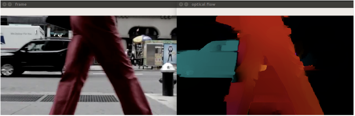

Screen Shot 2021-12-08 at 09.27.36.png

Farneback algorithm

Approximate some neighbors of each pixel with a polynomial, taking the second order of Taylor expansion

$I(x)\approx x^TAx+b^Tx+c$
We observe the differences in the approximated polynomials caused by object displacements

elif args.algorithm == 'farneback':
    method = cv2.calcOpticalFlowFarneback
    params = [0.5, 3, 15, 3, 5, 1.2, 0]  # default Farneback's algorithm parameters
    frames = dense_optical_flow(method, video_path, save, params, to_gray=True)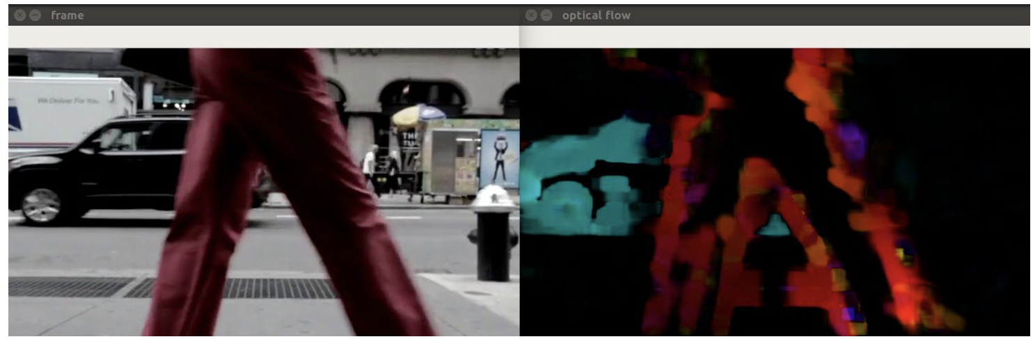

Screen Shot 2021-12-08 at 09.30.24.png

RLOF
- The intensity constancy assumption doesn’t fully reflect how the real world behaves.
- There are also shadows, reflections, weather conditions, moving light sources, and, in short, varying illuminations.
  
  $I(x,y,t)+mI(x,y,t)+c=I(x+u,y+v,t+1)$ with $m,c$ illumination parameters
```
elif args.algorithm == "rlof":
    method = cv2.optflow.calcOpticalFlowDenseRLOF
    frames = dense_optical_flow(method, video_path, save)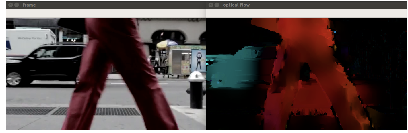
```

4. Camera Calibration and 3d reconstruction 6. Object Detection