Proba ML
5. Decision Theory
5.3 Frequentist Decision Theory

5.3 Frequentist decision theory

In frequentist decision theory, we don’t use prior and thus no posterior, so we can’t define the risk as the posterior expected loss anymore.

5.3.1 Computing the risk of an estimator

The frequentist risk of an estimator π\pi, applied to data xx sampled from the likelihood p(xθ)p(x|\theta):

R(θ,π)Ep(xθ)[(θ,π(x))]R(\theta,\pi) \triangleq \mathbb{E}_{p(x|\theta)}[\ell(\theta,\pi(x))]

Exemple

We estimate the true mean of a Gaussian. Let xnN(θ,σ2=1)x_n \sim \mathcal{N}(\theta^*,\sigma^2=1). We use a quadratic loss, so the risk is the MSE.

We compute the risk for different estimators, the MSE can be decomposed:

MSE(θ^θ)=Var[θ^]+bias2(θ^)\mathrm{MSE}(\hat{\theta}|\theta^*)=Var[\hat{\theta}] +bias^2(\hat{\theta})

with bias(θ^)=E[θ^θ]bias(\hat{\theta})=\mathbb{E}[\hat{\theta}-\theta^*].

  • π1=xˉ\pi_1=\bar{x} is the sample mean. This is unbiased, so its risk is:
MSE(π1θ)=σ2N\mathrm{MSE}(\pi_1|\theta^*)=\frac{\sigma^2}{N}
  • π2=median(D)\pi_2=\mathrm{median}(\mathcal{D}). This is also unbiased. One can show its variance is approximately:
MSE(π2θ)=π2N\mathrm{MSE}(\pi_2|\theta^*)=\frac{\pi}{2N}
  • π3\pi_3 returns the constant θ0\theta_0 so its biased is (θ0θ)(\theta_0-\theta^*), and its variance is zero. Hence:
MSE(π3θ)=(θ0θ)2\mathrm{MSE}(\pi_3|\theta^*)=(\theta_0-\theta^*)^2
  • πκ\pi_\kappa is the posterior mean under a N(θθ0,σ2/κ)\mathcal{N}(\theta|\theta_0,\sigma^2/\kappa) prior:
πκ(D)=NN+κxˉ+κN+κθ0=wxˉ+(1w)θ0\pi_\kappa(\mathcal{D})=\frac{N}{N+\kappa}\bar{x}+\frac{\kappa}{N+\kappa}\theta_0=w \bar{x}+(1-w)\theta_0

We can derive its MSE as follow:
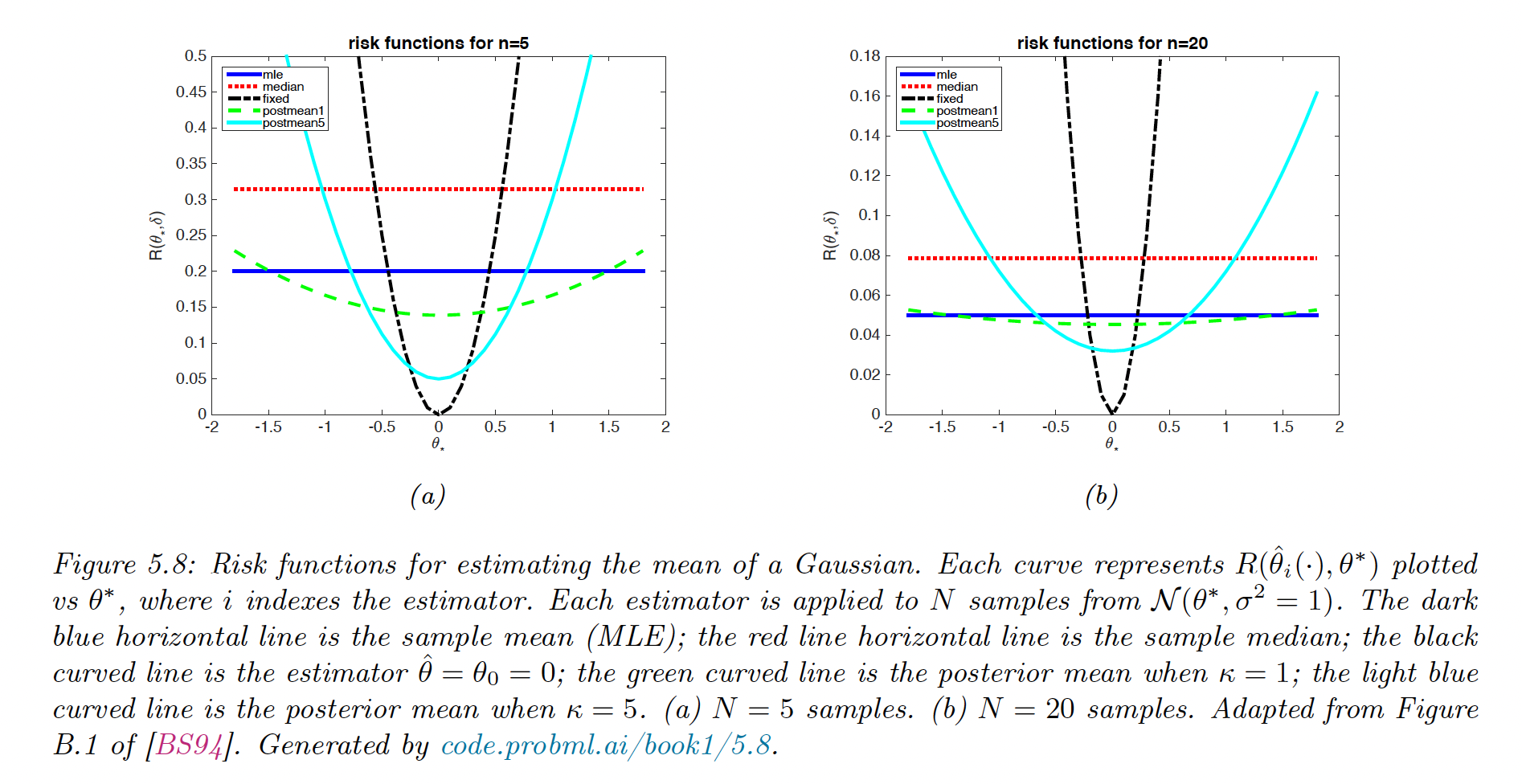
MSE(πkθ)=E[(wxˉ+(1w)θ0θ)2]=E[(w(xˉθ)+(1w)(θ0θ))2]=w2σ2N+(1w)2(θ0θ)2=1(N+κ)2(Nσ2+κ2(θ0θ)2)\begin{align} \mathrm{MSE}(\pi_k|\theta^*)&= \mathbb{E}[(w\bar{x}+(1-w)\theta_0-\theta^*)^2] \\ &= \mathbb{E}[(w(\bar{x}-\theta^*)+(1-w)(\theta_0-\theta^*))^2] \\ &= w^2 \frac{\sigma^2}{N}+(1-w)^2(\theta_0-\theta^*)^2 \\ &= \frac{1}{(N+\kappa)^2}(N\sigma^2+\kappa^2(\theta_0-\theta^*)^2) \end{align}

Screen Shot 2023-01-20 at 09.22.00.png

The best estimator depends on θ\theta^*, which is unknown. If θ0\theta_0 is far from θ\theta^*, the MLE is best.

Bayes risk

In general the true distribution of θ\theta is unknown, so we can’t compute R(θ,π)R(\theta,\pi). One solution is to average out all values of the prior π0\pi_0 for θ\theta. This is the Bayes risk or integrated risk.

R(π0,π)Eπ0(θ)[R(θ,π)]=ΘXp(xθ)(θ,π(x))dx  π0(θ)dθR(\pi_0,\pi) \triangleq \mathbb{E}_{\pi_0(\theta)}[R(\theta,\pi)]=\int_{\Theta} \int_{\mathcal{X}}p(x|\theta)\ell(\theta,\pi(x)) dx \;\pi_0(\theta)d\theta

The Bayes estimator minimizes the Bayes risk:

π(x)=arg minaπ0(θ)p(xθ)(θ,a)dθ=arg minap(θx)(θ,a)dθ\pi(x)=\argmin_a \int \pi_0(\theta)p(x|\theta)\ell(\theta,a)d\theta=\argmin_a\int p(\theta|x) \ell(\theta,a)d\theta

which corresponds to optimal policy recommended by Bayesian decision theory here.
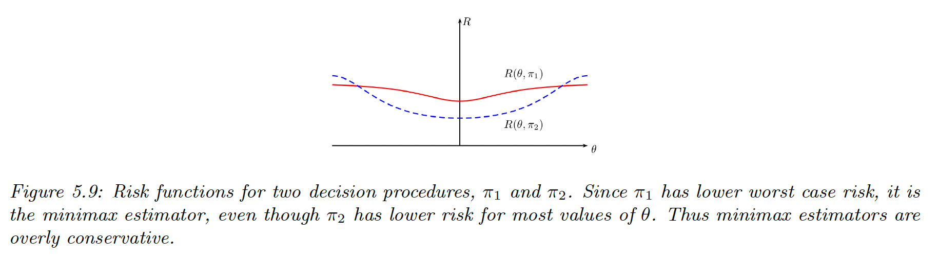
Maximum risk

To avoid using a prior in frequentist, we can define the maximum risk:

Rmax(π)supθR(θ,π)R_{max}(\pi) \triangleq \sup_\theta R(\theta,\pi)

To minimize the maximum risk, we use minimax πMM\pi_{MM}. Computing them can be hard though.

Screen Shot 2023-01-24 at 08.36.57.png

5.3.2 Consistent estimators

An estimator π:XNΘ\pi: \mathcal{X}^N\rightarrow\Theta is consistent when θ^(D)θ\hat{\theta}(\mathcal{D}) \rightarrow \theta^* as N+N\rightarrow +\infin, where the arrow is the convergence in probability.

This is equivalent to minimizing the 0-1 loss L(θ^,θ)=I(θ^θ)\mathcal{L}(\hat{\theta},\theta^*)= \mathbb{I}(\hat{\theta}\neq \theta^*).

An example of consistent estimator is the MLE.

Note that an estimator can be unbiased but not consistent, like π({x1,...,xN})=xN\pi(\{x_1,...,x_N\})=x_N. Since E[π(D)]=E[x]\mathbb{E}[\pi(\mathcal{D})]=\mathbb{E}[x] this is unbiased, but the sampling distribution of π(D)\pi(\mathcal{D}) doesn’t converge to a fix value so it is not consistent.

In practice, it is more useful to find some estimators that minimize the discrepancy between our empirical distribution pD(xD)p_\mathcal{D}(x|\mathcal{D}) and the estimated distribution p(xθ^)p(x|\hat{\theta}). If this discrepancy is the KL divergence, our estimator is the MLE.

5.3.3 Admissible estimators

π1\pi_1 dominates π2\pi_2 if:

θ,R(θ,π1)R(θ,π2)\forall\theta,R(\theta,\pi_1)\leq R(\theta,\pi_2)

An estimator is admissible when it is not dominated by any others.

In figure 5.8 above, we see that the risk of the sample median π2\pi_2 is dominated by the sample mean π1\pi_1.

However this concept of admissibility is of limited value, since π3(x)=θ0\pi_3(x)=\theta_0 is admissible even though this doesn’t even look at the data.