7.5 Singular Value Decomposition (SVD)
SVD generalizes EVD to rectangular matrices. Even for square matrices, an EVD does not always exist, whereas an SVD always exists.
7.5.1 Basics
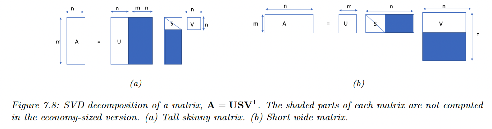
Any real matrix can be decomposed as:
with and orthogonal matrices (left and right singular vectors):
- is a matrix, containing the rank singular values .
The cost of computing the SVD is
7.5.2 Connection between EVD and SVD
If is real, symmetric, and positive definite, then the singular values are equal to the eigenvalues:
More generally, we have:
Hence:
- and
- and
- In the economy size SVD:
7.5.3 Pseudo inverse
The Moore-Penrose pseudo-inverse of is denoted and has the following properties:
If is square and non-singular, then
If and all columns of are linearly independent (i.e. is full-rank):
In this case, is the left inverse of (but not its right inverse):
We can also compute the pseudo-inverse using the SVD:
When , the right inverse of is:
and we have:
7.5.4 SVD and the range and null space
We show that the left and right singular vectors form an orthonormal basis for the range and nullspace.
We have:
where is the rank of .
Thus can be written as any linear combination of left singular vectors :
with dimension .
For the nullspace, we define as a linear combination of the right singular vectors for the zero singular values:
Then:
Hence:
with dimension .
We see that:
This is also written:
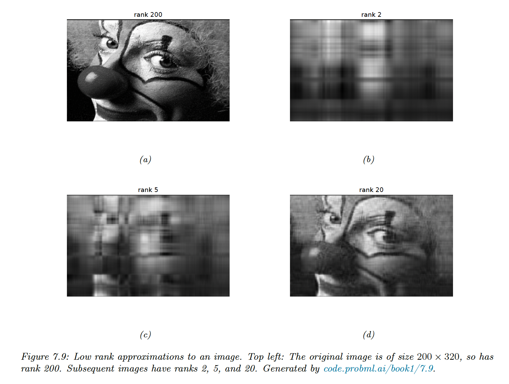
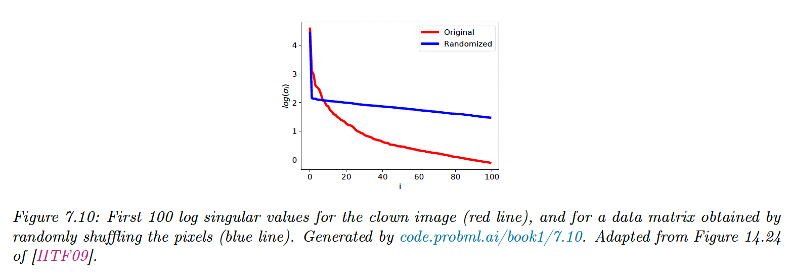
7.5.5 Truncated SVD
Let where we use the first columns. This can be shown to be the optimal rank approximation of in the sense of:
If , we incur some error: this is the truncated SVD.
The number of parameters needed to represent an matrix is .