Proba ML
4. Statistics
4.5 Regularization

4.5 Regularization

The main issue with MLE and ERM is that they pick parameters by minimizing the loss on the training set, which can result in overfitting.

With enough parameters, a model can match any empirical distribution. However, in most cases the empirical distribution is not the same as the true distribution. Regularization add a penalty term to the NLL.

L(θ,λ)=1Ni=1N(yn,θ,xn)+λC(θ)=1Ni=1Nlogp(ynxn,θ)λlogp(θ)\begin{align} \mathcal{L}(\theta,\lambda)&=\frac{1}{N}\sum^N_{i=1}\ell(y_n,\theta,x_n)+\lambda C(\theta) \\ &=-\frac{1}{N}\sum^N_{i=1} \log p(y_n|x_n,\theta) -\lambda \log p(\theta) \end{align}

by taking the log loss and the log prior for penalty term.

This is equivalent to minimizing the MAP:

θ^map=arg maxθlogp(θD)=arg maxθ[logp(Dθ)+logp(θ)const]\hat{\theta}_{map}=\argmax_{\theta} \log p(\theta|\mathcal{D})=\argmax_{\theta} [\log p(\mathcal{D}|\theta)+\log p(\theta) -\mathrm{const}]

4.5.1 MAP for Bernoulli distribution

If we observe just one head, θmle=1\theta_{mle}=1. We add a penalty to θ\theta to discourage extreme values.

With p(θ)Beta(a,b)p(\theta)\sim Beta(a,b), and a,b>1a,b>1, we encourage values of θ\theta near to the mean a/(a+b){a}/(a+b)

LL(θ)=logp(Dθ)+logp(θ)=N0logθ+N1log(1θ)+(a1)logθ+(b1)log(1θ)\begin{align} \mathrm{LL}(\theta)&=\log p(\mathcal{D}|\theta)+\log p(\theta) \\ &= N_0 \log\theta+ N_1 \log(1 - \theta) + (a-1)\log \theta + (b-1)\log (1-\theta) \end{align}

With the same method as the MLE, we find:

θ^map=N1+a1N+a+b2=N1+1N+2\hat{\theta}_{map}=\frac{N_1+a-1}{N+a+b-2}=\frac{N_1+1}{N+2}

By setting a=2,b=2a=2, b=2, we resolve the zero-count problem.

Regularization combines empirical data and prior knowledge.

4.5.2 MAP for MVN

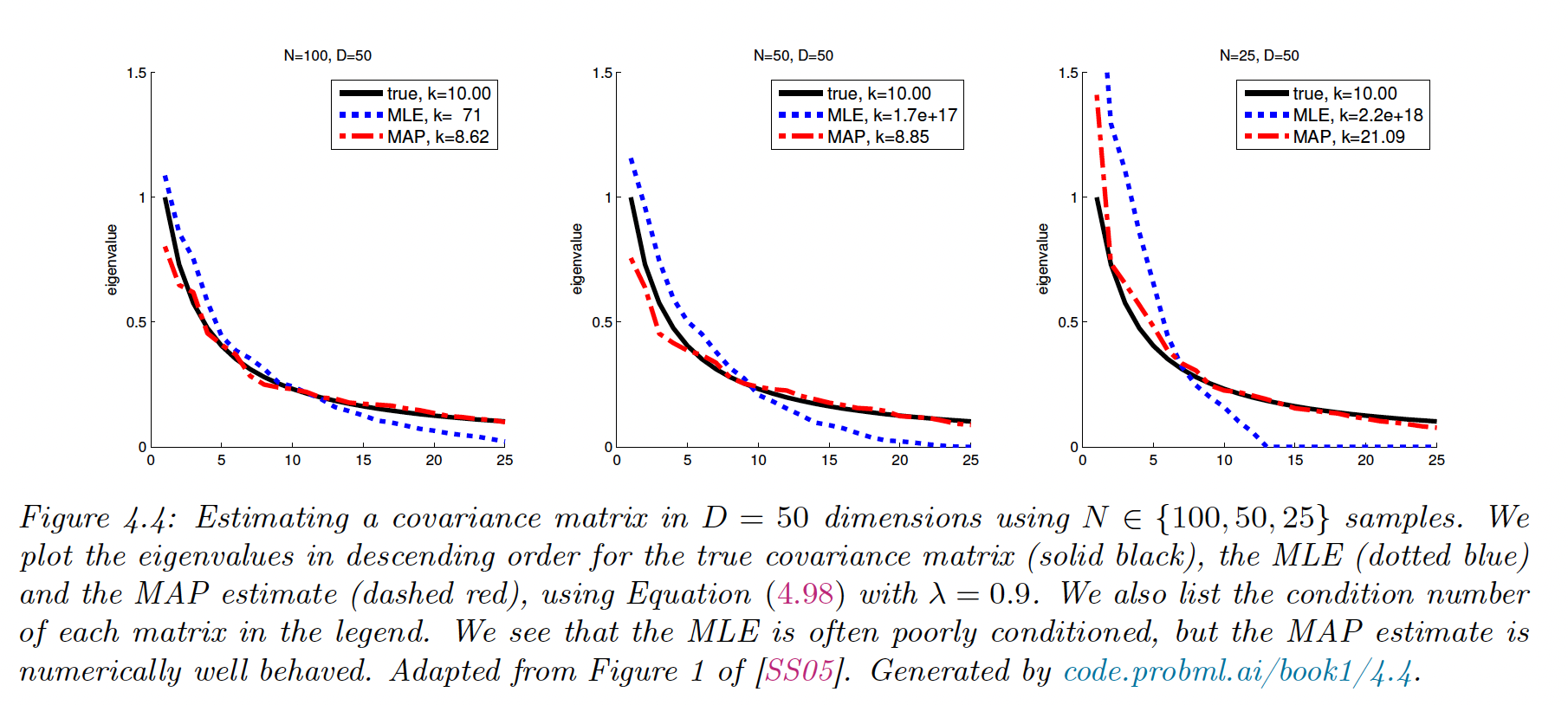
We showed that the MLE for covariance of a MVN is Σ^=1NSyˉ\hat{\Sigma}=\frac{1}{N}S_{\bar{y}}. In high dimensions, the scatter matrix can easily become singular. One solution is to perform MAP estimation.

A convenient prior to use for Σ\Sigma is the Wishart distribution (generalization of the Gamma distribution). The resulting MAP is:

Σ^map=S˘+SyˉN˘+N=N˘N˘+NS˘N˘+NN˘+NSyˉN=λΣ0+(1λ)Σ^mle\hat{\Sigma}_{map}=\frac{\breve{S}+S_{\bar{y}}}{\breve{N}+N}=\frac{\breve{N}}{\breve{N}+N}\frac{\breve{S}}{\breve{N}}+\frac{N}{\breve{N}+N}\frac{S_{\bar{y}}}{N}=\lambda \Sigma_0+(1-\lambda)\hat{\Sigma}_{mle}

where λ\lambda controls the amount of regularization.

If we set S˘=Ndiag(Σ^mle)\breve{S}=N \mathrm{diag}(\hat{\Sigma}_{mle}):

Σ^map(i,j)={Σ^mleifi=j(1λ)Σ^mleo.w.\hat{\Sigma}_{map}(i,j)=\begin{cases} \hat{\Sigma}_{mle}&\mathrm{if}\,i=j \\ (1-\lambda)\hat{\Sigma}_{mle} & o.w. \end{cases}

Off-diagonal elements are shrunk toward 0. λ\lambda can be chosen via cross-validation of via close form (implemented in scikit-learn LedoitWolf (opens in a new tab)).

The benefits of the MAP is to better behaved than MLE, with eigenvalues of the estimate closer to that of the true covariance matrix (the eigenvectors however are unaffected).

Screen Shot 2022-11-20 at 17.51.17.png

4.5.3 Weight decay

We saw that reducing the degree of the polynomial help the regression task. A more general solution is to add regularization to the regression coefficients.

w^map=arg minwNLL(w)+λw22\hat{w}_{map}=\argmin_w \mathrm{NLL}(w)+\lambda ||w||_2^2

where a higher λ\lambda means more pressure toward low coefficients and thus less flexibility for the model. This is ridge regression.

Screen Shot 2022-11-20 at 18.02.40.png

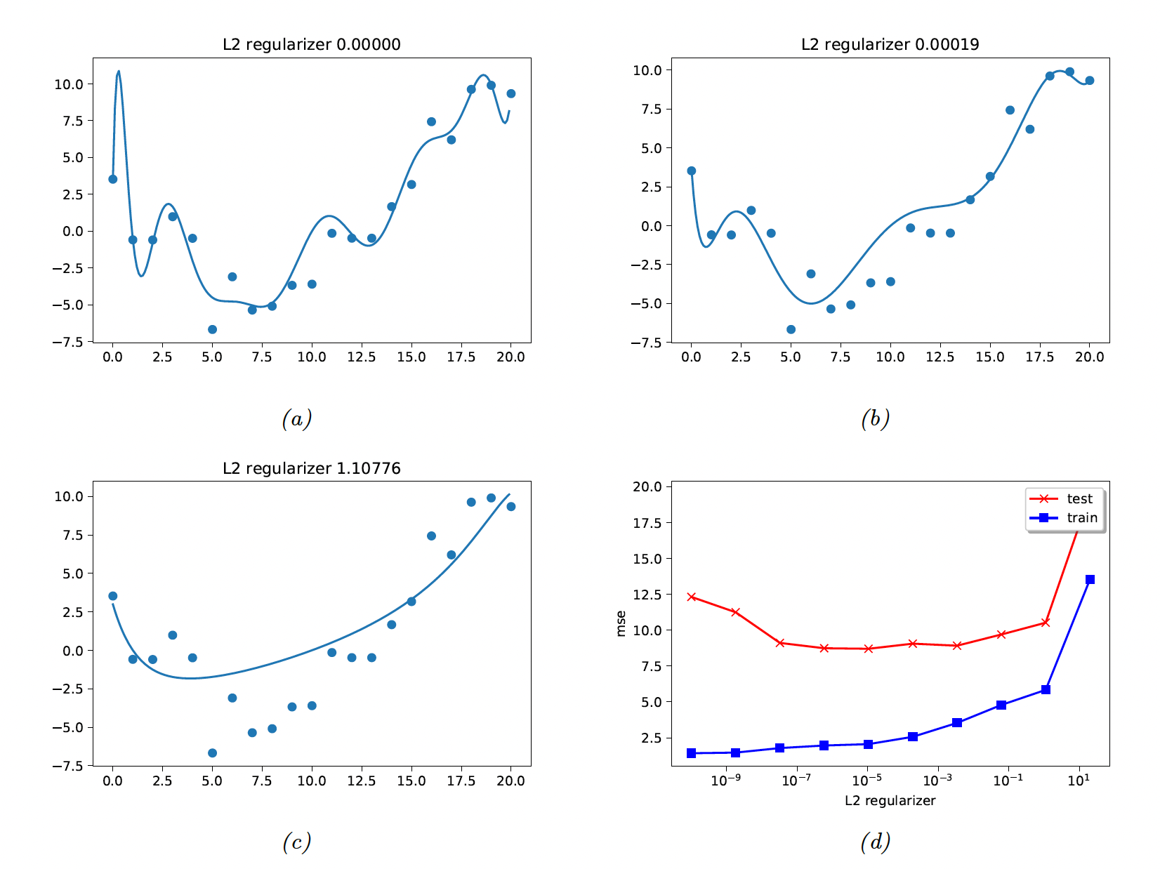
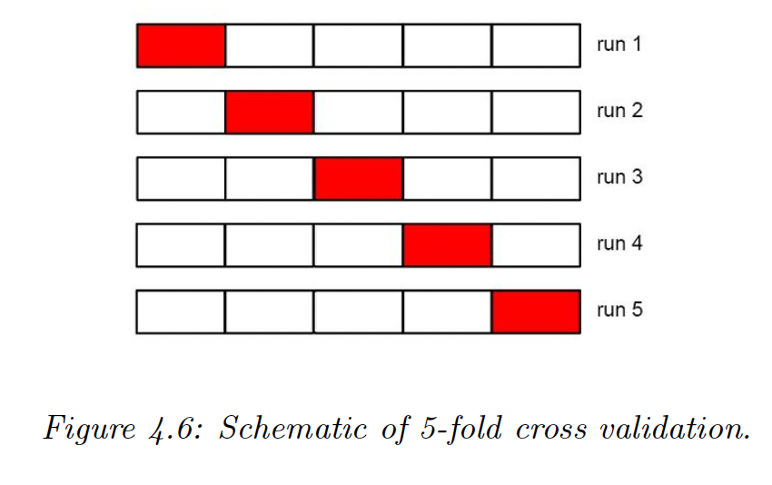
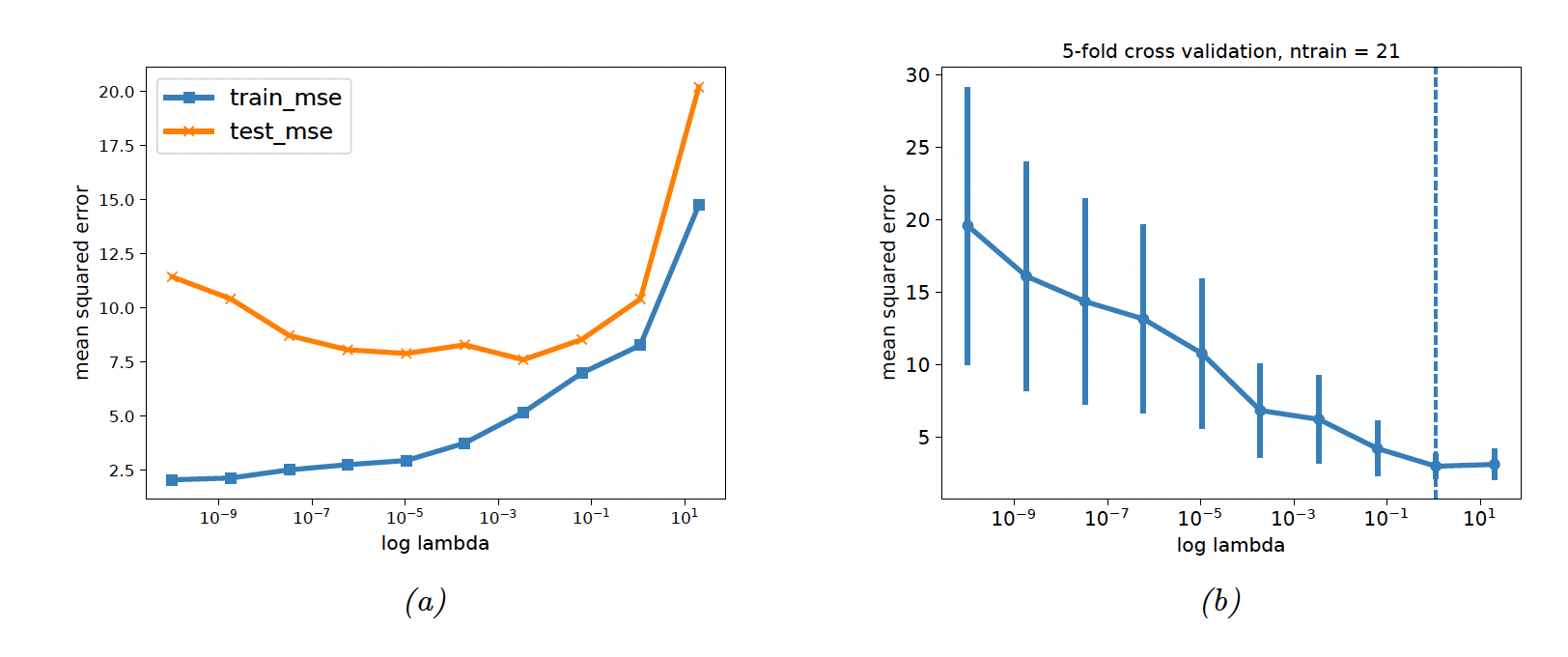
4.5.4 Picking 𝝺 by cross validation

We split the training data into KK folds and iteratively fit on all fold except one, used for validation.

Screen Shot 2022-11-20 at 18.09.55.png

We have

Rλ(θ,D)=1D(x,y)D(y,f(x,θ))+λC(θ)R_\lambda(\theta,\mathcal{D})=\frac{1}{|D|}\sum_{(x,y) \in \mathcal{D}} \ell(y,f(x,\theta))+\lambda C(\theta)

So

λ^=arg minλRλcv=arg minλ1Kk=1KR0(θ^λ(Dk),Dk)\hat{\lambda} =\argmin_\lambda R^{cv}_\lambda =\argmin_\lambda\frac{1}{K}\sum_{k=1}^K R_0(\hat{\theta}_{\lambda}(\mathcal{D}_{-k}),\mathcal{D}_k)

Finally

θ^=arg minθRλ^(θ,D)\hat{\theta}=\argmin_{\theta}R_{\hat{\lambda}}(\theta,\mathcal{D})

The standard error of our estimate is:

se=σ^n\mathrm{se}=\frac{\hat{\sigma}}{\sqrt{n}}

where σ^=Var[(y,f(x,θ^))]\hat{\sigma}=\mathrm{Var}[\ell(y,f(x,\hat{\theta}))]

Screen Shot 2022-11-20 at 18.31.46.png

4.5.7 Using more data

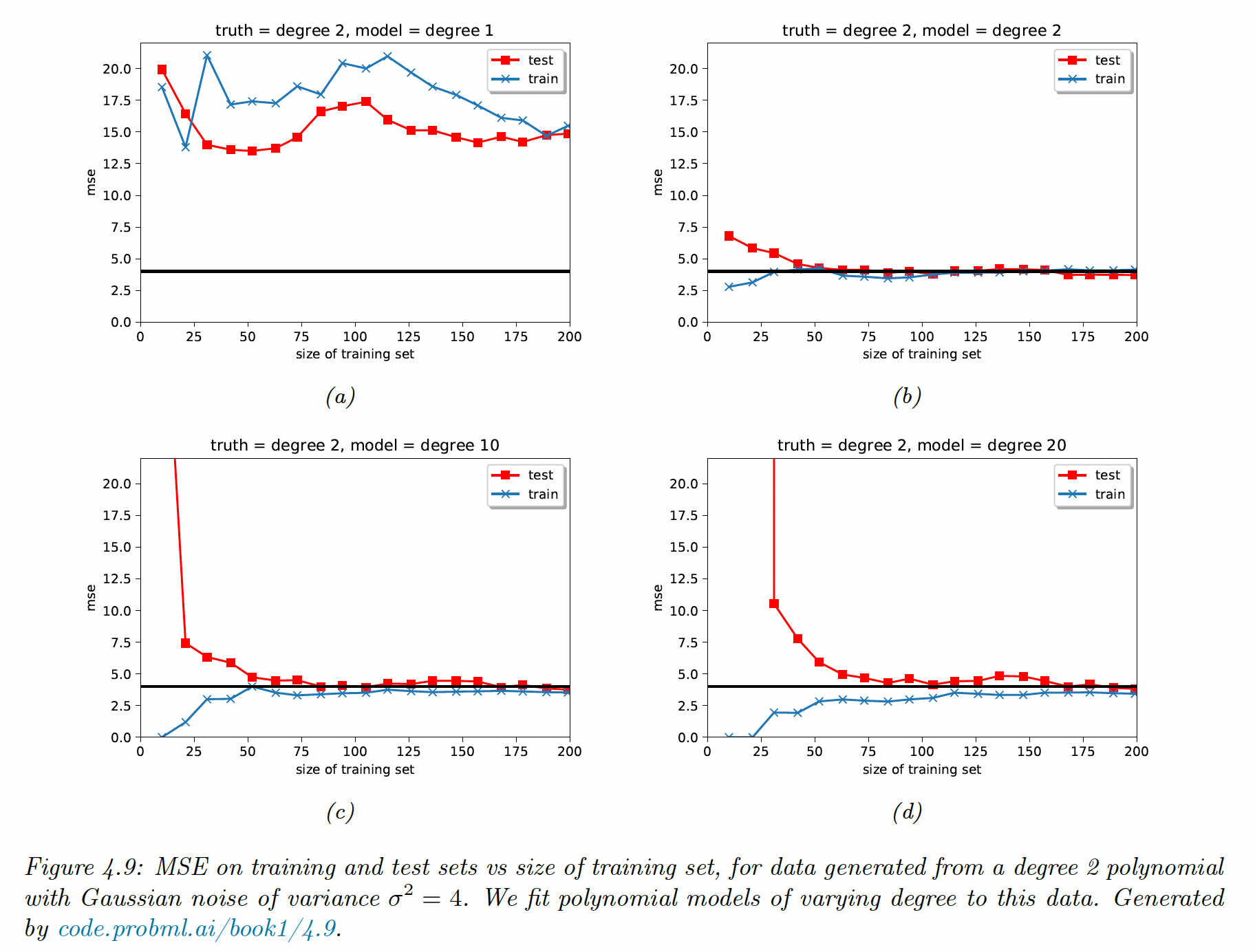
When a model is too simplistic, it fails to improve as the data grow. A overly complex model will end up converging toward the right solution if enough data is provided.

Screen Shot 2022-11-20 at 18.39.36.png