16.3 Kernel density estimation (KDE)

KDE is a form of non-parametric density estimation. This also a form of generative model, since it defines a probability distribution $p(\bold{x})$ that can be evaluated pointwise, and which can be sampled to generate new data

16.3.1 Density kernels

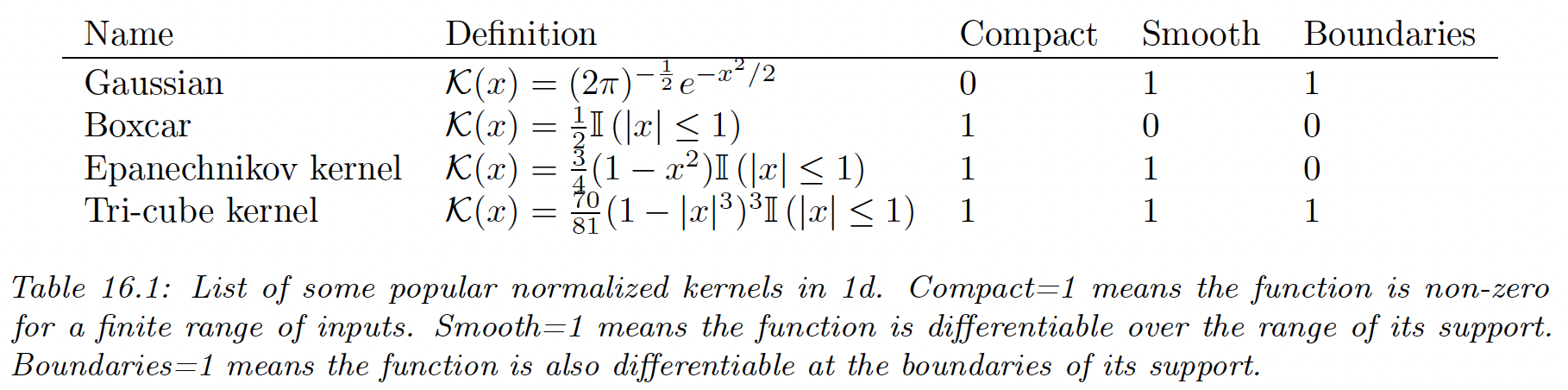
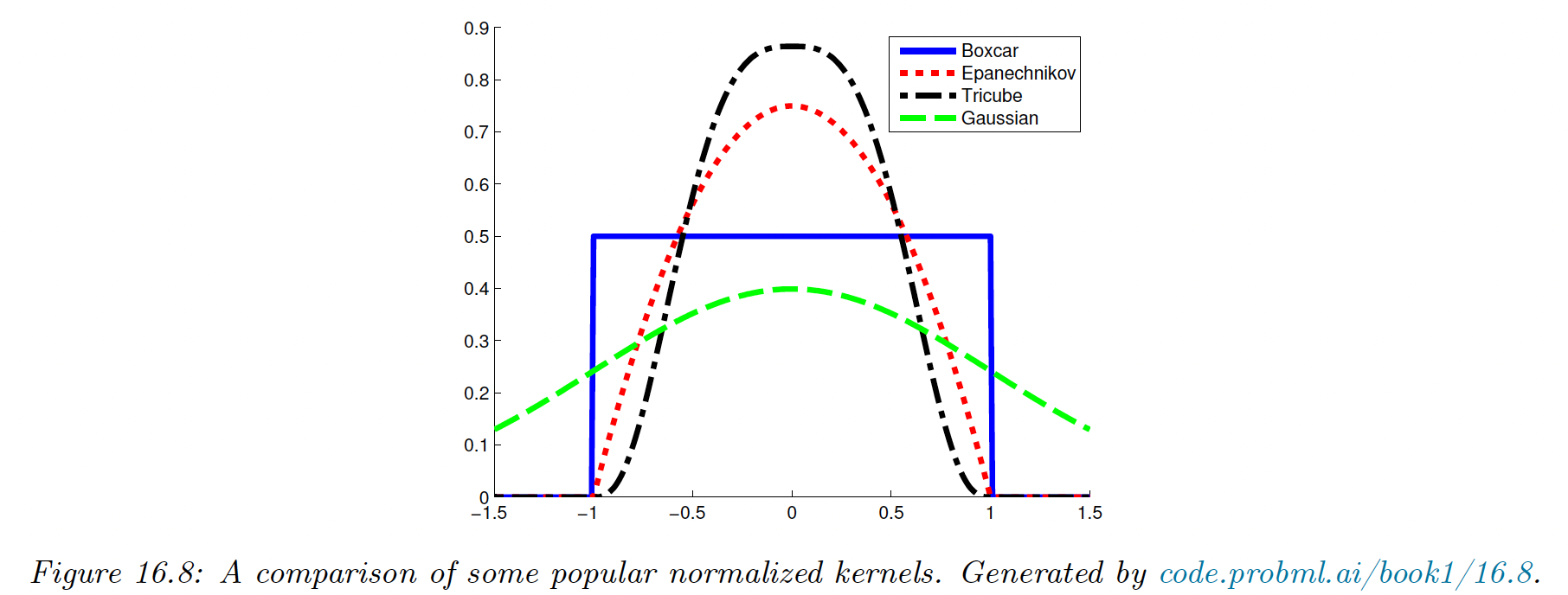
Density kernels are function $\mathcal{K}:\R \rightarrow \R_+$, such that $\int \mathcal{K}(x)dx=1$ and $\mathcal{K}(x)=\mathcal{K}(-x)$.

This latter symmetry property implies $\int x\mathcal{K}(x)dx=0$ and hence:

A simple example of such a kernel is the boxcar kernel, which is the uniform distribution around within the unit interval around the origin:

Another example is the Gaussian kernel:

We can control the width of the kernel by introducing a bandwidth parameter $h$:

We can generalize to vector valued inputs by defining a radial basis function (RBF) kernel:

In the case of the Gaussian kernel this becomes:

Although the Gaussian kernel is popular, it has unbounded support. Compact kernels can be faster to compute.

16.3.2 Parzen window density estimator

We now explain how to use kernels to define a nonparametric density estimate.

Recall the form of Gaussian mixture, with a fixed spherical Gaussian covariance and uniform mixture weights:

One problem with this model is that it requires specifying the number $K$ of clusters and their positions $\mu_k$.

An alternative is to allocate one cluster center per data point:

This can be generalized to:

This is called a Parzen window density estimator or kernel density estimator (KDE).

Its advantage over a parametric model is that no fitting is required (except for choosing $h$) and there is no need to select the clusters.

The drawback is that it takes a lot of memory and a lot of time to evaluate.

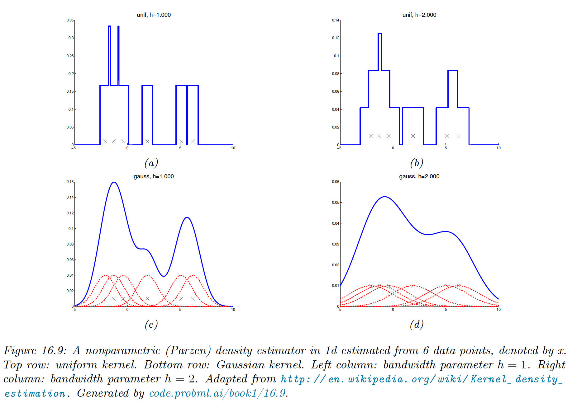
The resulting model using the boxcar kernel simply count the number of points within a window of size $h$. The Gaussian kernel gives a smoother density.

16.3.3 How to choose the bandwith parameter

The bandwidth parameter $h$ controls the complexity of the model.

In 1d data, if we assume the data has been generated from a Gaussian distribution, one can show the bandwidth minimizing the frequentist risk is given by:

We can compute a robust approximation to the standard deviation by first computing the median absolute deviation (MAD):

and then using $\hat{\sigma}=1.4826 \,\mathrm{MAD}$.

If we have $D$ dimension, we can estimate each $h_d$ separately for each dimension and then set:

16.3.4 From KDE to KNN classification

We previously discussed the $K$ neighbor classifier as a heuristic approach to classification. Interestingly, we can derive it as a generative classifier in which the class conditional densities $p(\bold{x}|y=c)$ are modeled using a KDE.

Rather than a fixed bandwidth a counting the points within a hypercube centered on a datapoint, we allow the bandwidth to be different for each point.

We “grow” a volume around $\bold{x}$ until we captured $K$ points, regardless of their class label. This is called a balloon density kernel estimator.

Let the resulting volume have size $V(\bold{x})$ (this was previously $h^D)$ and let there $N_c(\bold{x})$ example of the class $c$ in this volume. We can then estimate the class conditional density:

where $N_c$ is the total number of point with class labels $c$ in the dataset.

If we take the class prior to be $N_c/N$, we have the posterior:

16.3.5 Kernel regression

Just as KDE can be use for generative classifiers, it can also be used as generative models for regression.

16.3.5.1 Nadaraya-Watson estimator for the mean

In regression, our goal is to compute:

If we use a MVN for $p(\bold{x},y|\mathcal{D})$, we derive a result which is equivalent to linear regression.

However, the Gaussian assumption on $p(\bold{x},y|\mathcal{D})$ is rather limiting. We can use KDE to more accurately approximate this joint density:

Hence, using the previous kernel properties:

where:

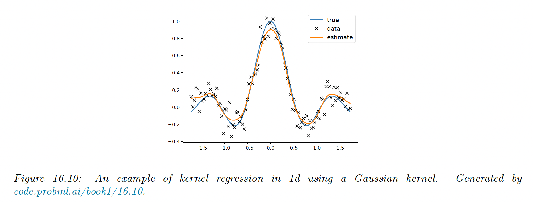
We see that the prediction is just a weighted sum of the training labels, where the weights depend on the similarity between $\bold{x}$ and the stored training points.

This method is called kernel regression, kernel smoothing, or the Nadaraya-Watson (N-W) model.

16.3.5.2 Estimator for the variance

Sometimes it can be useful to compute the predictive variance, as well as the predictive mean. We can do this by noting that:

where $\mu(\bold{x})=\mathbb{E}[y|\bold{x},\mathcal{D}]$ is the Nadara-Watson estimate.

If we use a Gaussian kernel with variance $\sigma^2$, we can compute:

where we used the fact that:

Finally:

16.3.5.3 Locally weighted regression

We can drop the normalization term to get:

Rather than interpolating the stored labels $y_n$, we can fit a locally linear model around each training point:

This is called locally linear regression (LLR), or locally-weighted scatterplot smoothing (LOWESS or LOESS).

This is often used when annotating scatter plots with local trend lines.