8.3 Second-order methods

First-order methods only exploit the gradient of the loss function, which is cheap to compute but can be imprecise. Second-order methods leverage the curvature of the loss using the Hessian.

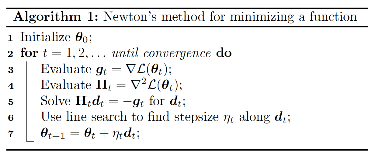
8.3.1 Newton’s method

The classic second-order method is Newton’s method, whose update is:

where $H_t$ is assumed positive-definite. The intuition is that $H^{-1}$ “undoes” the skewness in the local curvature.

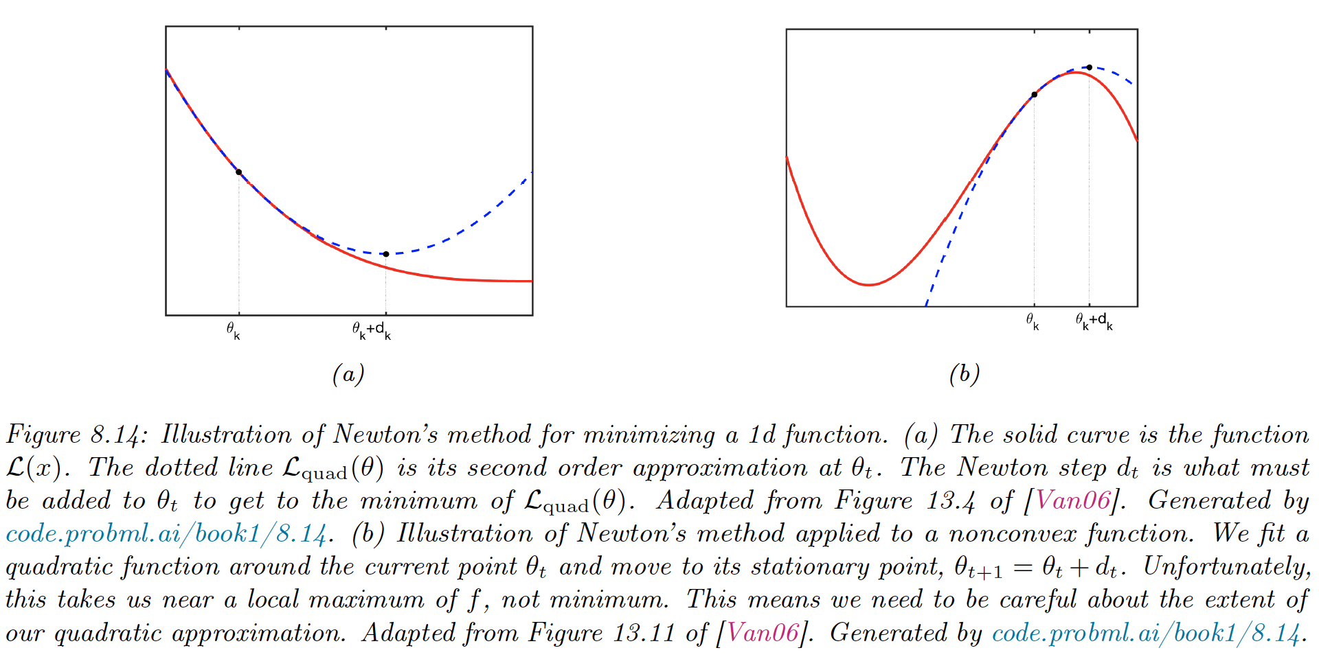
To see why, consider the Taylor series approximation of $\mathcal{L(\theta)}$ around $\theta_t$:

The differential w.r.t $\theta$ gives:

8.3.2 BFGS

Quasi-Newton methods iteratively build up an approximation to the Hessian, using information about the gradient at each step:

with $\bold{s}_t=\theta_t-\theta_{t-1}$ and $\bold{y}_t=\bold{g}_t-\bold{g}_{t-1}$

If $B_0$ is positive definite and the step size $\mu$ is chosen via line search satisfying the Armiko condition and the curvature condition:

with $c_2\in[c,1]$, then $B_{t+1}$ remains positive definite.

Typically, $B_0=I$.

Alternatively, BFGS can iteratively update an approximate the inverse of the Hessian:

Since storing the Hessian approximation still takes $O(D^2)$ space, for very large problems the limited memory (L-BFGS) is preferred.

Rather than storing $B_t$, we store the $M$ most recent $(s_t,y_t)$ and then approximate $H_t^{-1} \bold{g}_t$ by performing a sequence of inner products with the stored $\bold{s}_t$ and $\bold{y}_t$ vectors.

$M$ between 5-20 is often sufficient.

8.3.3 Trust region methods

If the objective function is non-convex, then the Hessian may not be positive definite, so $\bold{d}_t=-H_t\bold{g}_t$ may not be the descent direction. In general, any time the quadratic approximation made by Newton’s method is invalid, we are in trouble.

However, there is usually a local region $\mathcal{R}_t$ around the current iterate where we can safely approximate the objective by a quadratic.

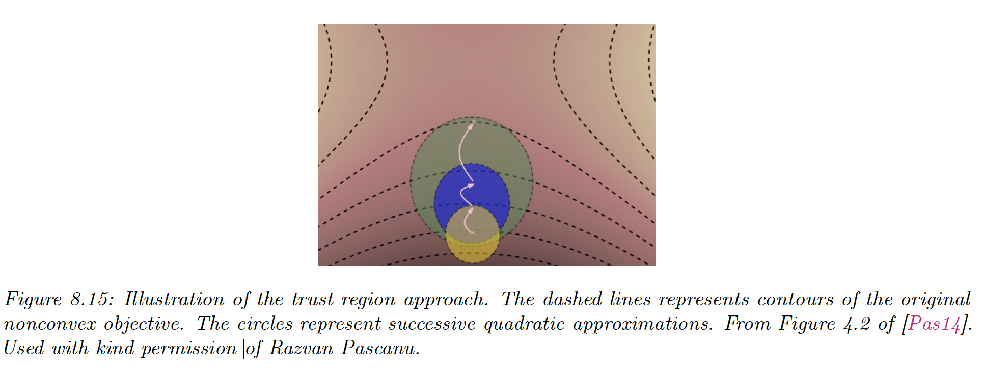
Let $M(\delta)$ the approximation to the objective, where $\delta=\theta-\theta_t$. At each step, we solve:

this is called trust-region optimization.

We usually assume $M_t$ is a quadratic approximation:

We assume that the region is a ball:

The constraint problem becomes an unconstrained one:

for some Lagrange multiplier $\lambda >0$.

We can solve this using:

This is called Tikhonov regularization, adding a sufficiently large $\lambda I$ ensure that the resulting matrix is always positive definite.

See Beyond auto-differentiation (opens in a new tab) from Google AI using trust region and quadratic approximations.