7.2 Matrix multiplication
The product of and is with:
Note that the number of columns of must match the number of rows of .
Matrix multiplication complexity averages , faster methods exists (like BLAS) and hardware parallelizing the computation, like TPU or GPU.
- Matrix multiplication is associative:
- Matrix multiplication is distributive:
- In general, it is not commutative:
7.2.1 Vector-vector products
Inner product
Given two vectors , their size is . The inner product is the scalar:
Note that
Outer product
Given two vectors and (they no longer have the same size), the outer product is a matrix :
7.2.2 Vector-matrix products
Given matrix and , the product is
This can be viewed as inner product on rows:
Or linear combination on columns:
In this latter view, A is a set of basis vectors defining a linear subspace.
7.2.3 Matrix-matrix products
The main view is a inner product between row vectors of and columns vectors of :
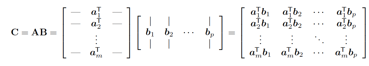
If and , then
7.2.4 Matrix manipulations
Summing slices
Let , we can average rows of by pre-multiplying a vector of ones:
Conversely, we can average columns by post-multiplying.
Hence, the overall mean is given by:
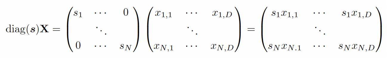
Scaling
If we pre-multiply by a diagonal matrix , we scale each row by :
Conversely, we scale columns by post-multiplying with the diagonal matrix
Therefore, the normalization operation can be written:
where is the empirical mean vector and the empirical standard deviation vector.
Scatter matrix
The sum of squares matrix is:
The scatter matrix is:
The Gram matrix is:
The square pairwise distance between and is:
This can also we written as:
where
7.2.5 Kronecker products
and , then the Kronecker product belongs to :
Some useful properties:
7.2.6 Einstein summation
Einsum consists in removing the operator for matrix and tensor products:
And for more complex operations:
Einsum can perform computations in an optimal order, minimizing time and memory allocation.