7.7 Solving systems of Linear Equation

We can formulate linear equations in the form of $A\bold{x}=\bold{b}$.

If we have $m$ equations and $n$ unknowns, then $A$ will be a $m\times n$ matrix and $\bold{b}$ a $m\times 1$ vector.

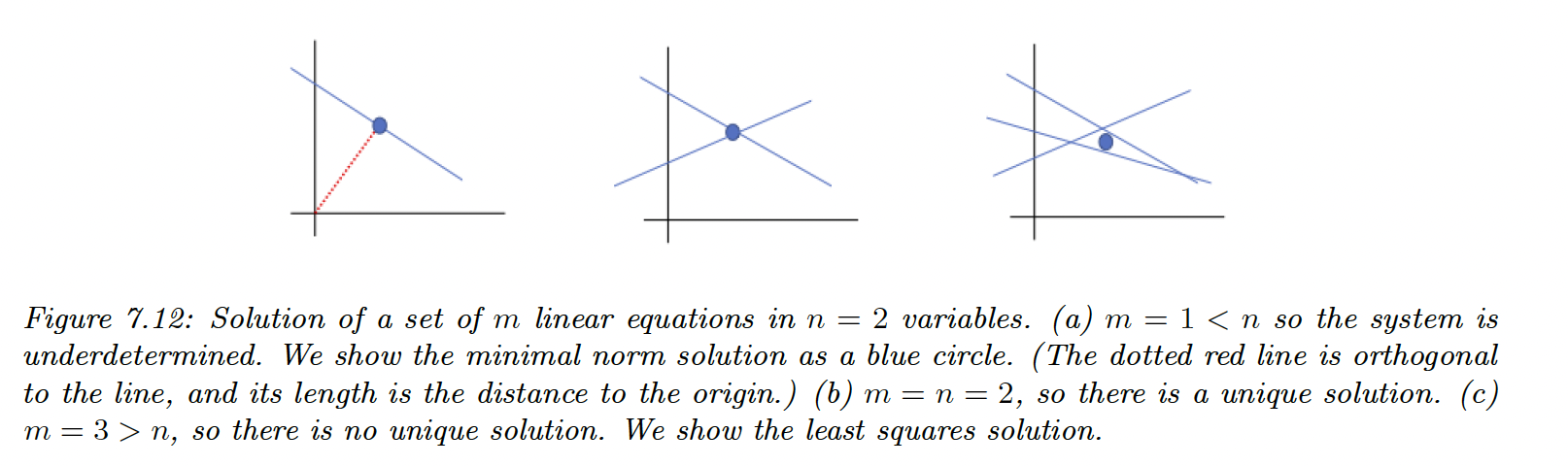
• If $m=n$ and $A$ is full rank, there is a single unique solution
• If $m<n$ the system is underdetermined so there is no unique solution
• If $m>n$ the system is overdetermined, not all the lines intersect at the same point

7.7.1 Solving square systems

When $m=n$, we can solve the LU decomposition for $\bold{x}$.

The point is that $L$ and $U$ are triangular, so we don’t need to compute the inverse and can use back substitution instead. For $L^{-1}\bold{b}=\bold{y}$

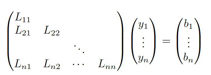
We start by solving $y_1=b_1/L_{11}$, then we substitute it into $L_{12}y_1+L_{22}y_2=b_2$ and iterate.

Once we have $\bold{y}$, we can apply the same computation for $x=U^{-1}\bold{y}$.

7.7.2 Solving under-constrained systems (least norm estimation)

We assume $m<n$ and $A$ to be full-rank, so there are multiple solutions:

Where $\bold{x}_p$ is any solution. It is standard to pick the solution minimizing the $\ell_2$ regularization:

We can compute the minimal norm solution using the right pseudo inverse:

We can also solve the constrained optimization problem by minimizing the norm:

Therefore:

Finally we find the right pseudo inverse again:

7.7.3 Solving over-constrained systems (least square estimation)

If $m>n$, we’ll try to find the closest solution satisfying all constrained specified by $A\bold{x=b}$, by minimizing the least square objective:

We know that the gradient is:

Hence the solution is the OLS:

With $A^\dagger=(A^\top A)^{-1} A^\top$ the left pseudo inverse.

We can check that this solution is unique by showing that the Hessian is positive definite:

Which is positive definite if $A$ is full-rank since for any $\bold{v}>\bold{0}$ we have: