Proba ML
8. Optimization
8.6 Proximal Gradient Methods

8.6 Proximal gradient method

We are often interested in optimizing an objective of the form:

L(θ)=Ls(θ)+Lr(θ)\mathcal{L}(\theta)=\mathcal{L}_s(\theta)+\mathcal{L}_r(\theta)

where:

  • Ls\mathcal{L}_s is a differentiable (smooth) loss, like the NLL
  • Lr\mathcal{L}_r is a convex loss but may not be differentiable, like the 1\ell_1 norm or an indicator function that is infinite when constraints are violated.

One way to solve this is to use a Proximal gradient method: take a step size μ\mu in the gradient direction and then project the result in the constraints space respecting Lr\mathcal{L}_r:

θt+1=proxLr,μ(θtμtLs(θt))\theta_{t+1}=\mathrm{prox}_{\mathcal{L_r}, \mu}(\theta_t-\mu_t \nabla \mathcal{L}_s(\theta_t))

where:

proxLr,μ=arg minz(Lr(z)+12μzθ22)\mathrm{prox}_{\mathcal{L}_r, \mu} = \argmin_z \Big(\mathcal{L}_r(z) + \frac{1}{2\mu}||z-\theta||^2_2 \Big)

We can rewrite the proximal operator as a constraint optimization problem:

arg minzLr(z)s.tzθ2ρ\argmin_z \mathcal{L}_r(z)\quad s.t \quad ||z-\theta||_2\leq \rho

Thus the proximal function minimizes the rough loss while staying close to the current iterate θt\theta_t.

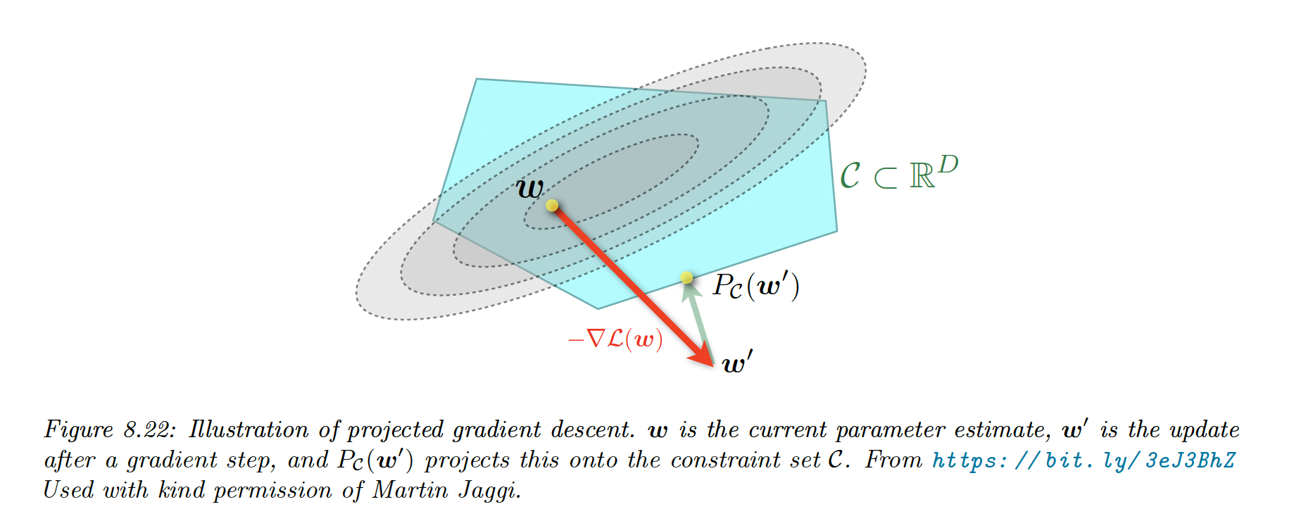
8.6.1 Projected gradient descent

We want to optimize:

arg minθLs(θ)s.t.θC\argmin_{\theta}\mathcal{L}_s(\theta) \quad s.t. \quad \theta \in \mathcal{C}

where C\mathcal{C} is a convex set.

We can have box constraints, with C={θ:lθu}\mathcal{C}=\{\theta :l \leq \theta \leq u \}

In unconstrained settings, this becomes:

L(θ)=Ls(θ)+Lr(θ)\mathcal{L}(\theta)=\mathcal{L}_s(\theta)+\mathcal{L}_r(\theta)

with:

Lr(θ)=IC(θ)={0if  θCo.w\mathcal{L}_r(\theta)=I_\mathcal{C}(\theta)= \begin{cases} 0 \quad \mathrm{if} \;\theta \in \mathcal{C} \\ \infin \quad o.w \end{cases}

We can solve that with the proximal gradient operator:

projC(θ)=arg minθCθθ2\mathrm{proj}_\mathcal{C}(\theta)=\argmin_{\theta' \in \mathcal{C}} ||\theta'-\theta||_2

Screen Shot 2023-06-03 at 18.14.33.png

In the box constraints example, the projection operator can be computed element-wise:

projC(θ)d={ldif  θdldθdif  ldθdududif  udθd\mathrm{proj}_{\mathcal{C}}(\theta)_d= \begin{cases} l_d \quad \mathrm{if}\; \theta_d\leq l_d \\ \theta_d \quad \mathrm{if}\; l_d \leq \theta_d \leq u_d \\ u_d \quad \mathrm{if}\; u_d \leq \theta_d \end{cases}

8.6.2 Proximal operator for the L1-norm regularizer

A linear predictor has the form f(x,θ)=dθdxdf(x,\theta)=\sum_d \theta_d x_d.

We can foster model interpretability and limit overfitting by using feature selection, by encouraging weight to be zero by penalizing the 1\ell_1 norm:

θ1=dθd||\theta||_1=\sum_d |\theta_d|

This induces sparsity because if we consider 2 points: θ=(1,0)\theta=(1,0) and θ=(1/2,1/2)\theta'=(1/\sqrt{2},1/\sqrt{2}), we have θ2=θ2||\theta||_2=||\theta'||_2 but θ1<θ1||\theta||_1 < ||\theta'||_1.

Therefore the sparse solution θ\theta is cheaper when using the 1\ell_1 norm.

If we combine our smooth loss with the regularizer we get:

L(θ)=NLL(θ)+λθ1\mathcal{L}(\theta)=NLL(\theta)+\lambda||\theta||_1

We can optimize this with the proximal operator, in a element-wise fashion:

proxλ(θ)=arg minzz+12λ(zθ)2\mathrm{prox}_\lambda(\theta)=\argmin_{z} |z| + \frac{1}{2\lambda} (z-\theta)^2

In section 11.4.3, we show that the solution is given by the soft threshold operator:

proxλ(θ)={θ+λif  θλ0if  θλθλif  θλ\mathrm{prox}_\lambda(\theta)= \begin{cases} \begin{align} \theta + \lambda \quad &\mathrm{if}\; \theta \leq -\lambda \\ 0 \quad &\mathrm{if}\; |\theta|\leq \lambda \\ \theta -\lambda \quad &\mathrm{if} \;\theta\geq \lambda \end{align} \end{cases}

8.6.3 Proximal operator for quantization

In some applications like edge computing, we might want to ensure the parameters are quantized.

We define a regularizer measuring the distance between the parameter and its nearest quantized version:

Lr(θ)=arg minθ0C={1,+1}θθ01\mathcal{L}_r(\theta)=\argmin_{\theta_0\in\mathcal{C=\{-1,+1\}}}||\theta-\theta_0||_1

In the case C={1,+1}D\mathcal{C}=\{-1,+1\}^D, this becomes:

Lr(θ)=d=1Darg minθ0,d{1,+1}θdθ0,d\mathcal{L_r}(\theta)=\sum_{d=1}^D \argmin_{\theta_{0,d}\in \{-1,+1\}}|\theta_d-\theta_{0,d}|

We solve this with proximal gradient descent, in which we treat quantization as a regularizer: this is called ProxQuant.

The update becomes:

θ~t=proxλ,Lr(θtμtLs(θt))\tilde{\theta}_t=\mathrm{prox}_{\lambda, {\mathcal{L}_r}}(\theta_t-\mu_t \nabla \mathcal{L}_s(\theta_t))

8.6.4 Incremental (online) proximal methods

Many ML problems have an objective function that is the sum of losses, one per example: these problems can be solved incrementally, with online learning.

It is possible to extend proximal methods to these settings, the Kalman Filter is one example.