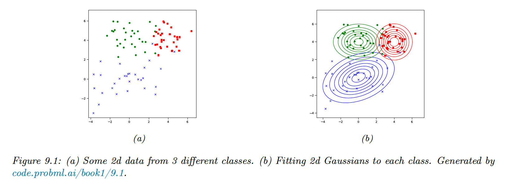
9.2 Gaussian Discriminant Analysis

The GDA is a generative classifier where the class conditional densities are multivariate Gaussian:

The corresponding class posterior has the form:

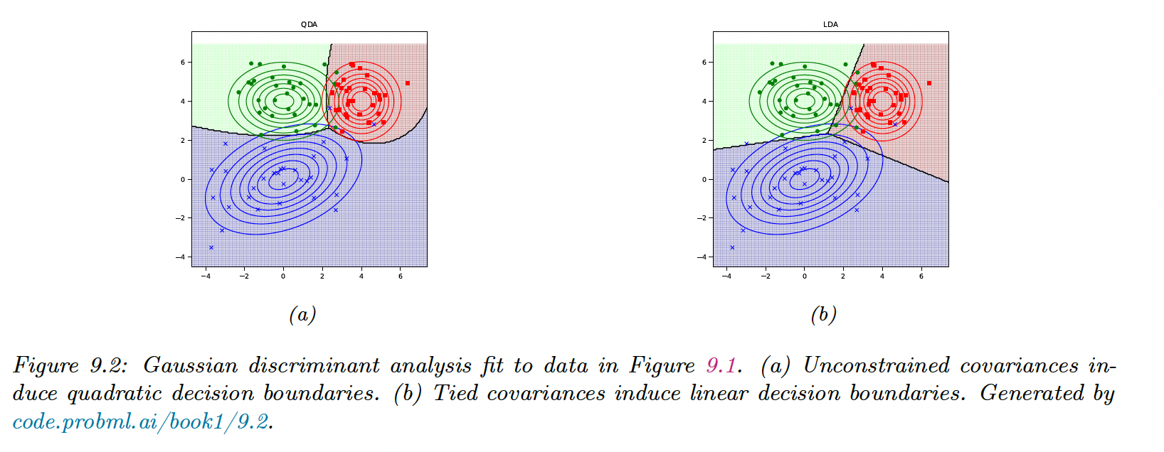
9.2.1 Quadratic decision boundaries

The log posterior over the class labels is:

This is called the discriminant function. The decision function between two classes, $c$ , and $c'$, is a quadratic function of $x$.

This technique is called Quadratic Discriminant Analysis (QDA).

9.2.2 Linear decision boundaries

We now consider the case of shared covariance, $\Sigma_c=\Sigma$:

$\kappa$ is a residual term across classes that can be removed.

This is called the Linear Discriminant Analysis (LDA).

9.2.3 Connection between LDA and Logistic Regression

From the LDA equation, we can write:

• In LDA, we first fit the Gaussians (and class prior) to fit the joint likelihood $p(x,y|\theta)$, then we use $\theta$ to derive $w_c=[\gamma_c,\beta_c]$
• In Logistic Regression, we estimate $w$ directly to maximize the conditional likelihood $p(y|x,\theta)$

In the binary case, this resume to:

With:

And by setting:

We end up with the binary logistic regression:

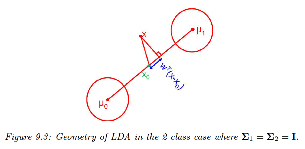
The MAP decision rule is:

In the case where $\pi_0=\pi_1$ and $\Sigma=\sigma^2I$, we end up with projecting $x$ on the $w=\sigma^{-2}(\mu_0-\mu_1)$ line and compare it to the centroid, $x_0$.

9.2.4 Model fitting

We now discuss how to fit the GDA model using MLE. The likelihood is:

Hence the log-likelihood is:

We can optimize $\pi_c$ and $(\mu_c,\Sigma_c)$ separately:

• From section 4.2.4, we have that the MLE of the prior is $\hat{\pi}_c=\frac{N_c}{N}$
• From section 4.2.6, the MLE for the Gaussian is:

Unfortunately, the MLE for $\hat{\Sigma}_c$ can easily overfit if $N_c<D$. Below are some workarounds.

9.2.4.1 Tied covariance

If we tied covariance matrices $\Sigma_c=\Sigma$, we get linear boundaries. This also allows pooling from all samples:

9.2.4.2 Diagonal covariance

If we force $\Sigma_c$ to be diagonal, we reduce the number of parameters from $O(C D^2)$ to $O(CD)$, which avoids the overfitting problem. However, we lose the ability to capture the correlation between features (this is the Naive Bayes assumption).

We can restrict further the model using a tied diagonal matrix: this is the diagonal LDA.

9.2.4.3 MAP estimation

Forcing the covariance to be diagonal is a rather strong assumption. Instead, we can perform a MAP estimation from section 4.5.2:

This technique is called regularized discriminant analysis (RDA).

9.2.5 Nearest Centroid Classifier

If we assume a uniform prior over classes, we compute the most probable labels as:

This is called the nearest centroid classifier, where the distance is measured using squared Mahalanobis distance.

We can replace this distance with any other distance metrics:

We can learn distance metrics with one simple approach:

The class posterior becomes:

We can optimize $W$ using gradient descent applied to the discriminative loss. This is called nearest class mean metric learning.

This technique can be used for one-shot learning of new classes since we just need to see a single labeled $\mu_c$ per class (assuming we have a good $W)$.

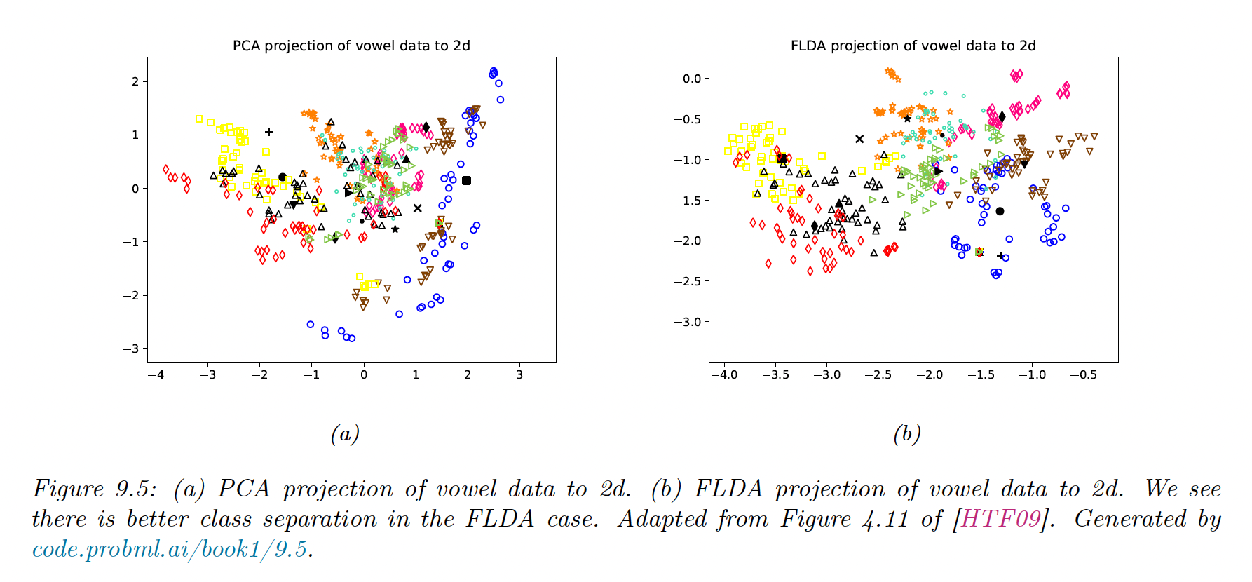
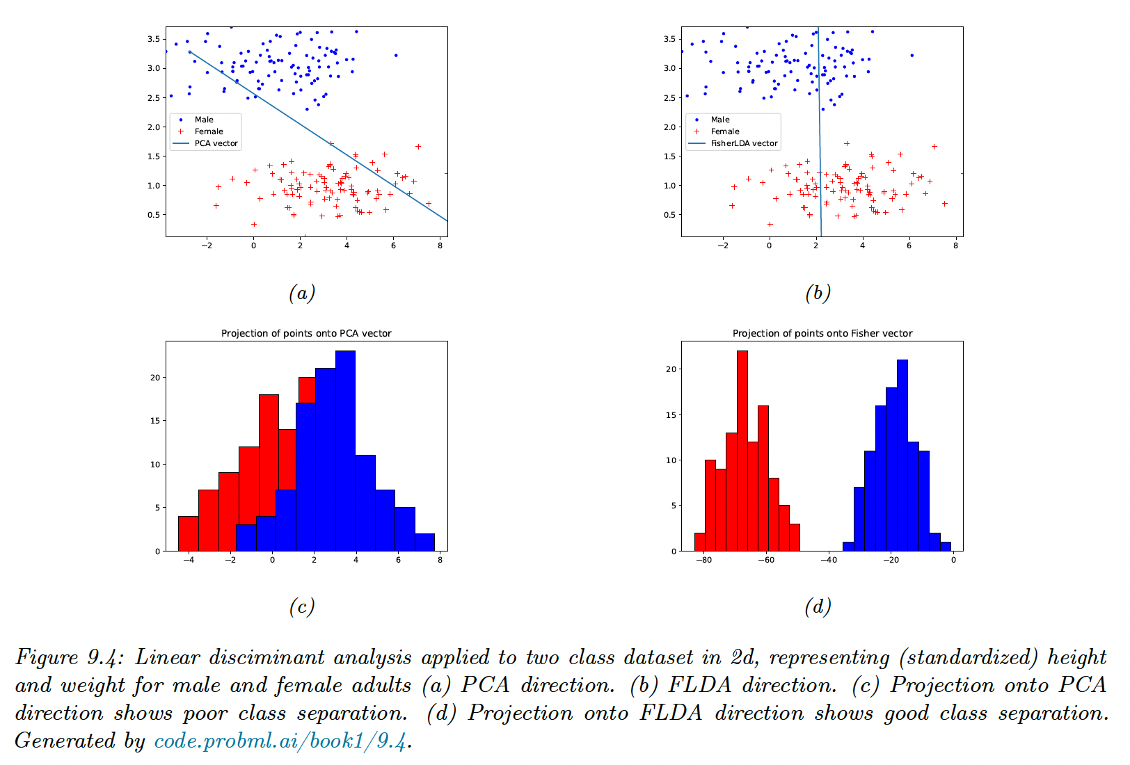
9.2.6 Fisher LDA

Discriminant analysis is a generative approach to classification, that requires fitting MVN to the feature. This might be problematic in high dimensions.

An alternative could be to reduce the features to $z\in\mathbb{R}^K$ and then to fit MVN, by finding $W\in\mathbb{R}^{K\times D}$ so that $z=Wx$ .

• The simplest way is using a PCA, but this is a non-supervised technique, and not taking the labels into account could lead to suboptimal low-dimensional features
• Alternatively, we could use a gradient-based method to optimize the log-likelihood, derived from the posterior in the low dimensional space, as we did with the nearest class mean metric learning
• A third approach relies on eigenvalues decomposition, by finding $W$ so that the low dimensional data can be classified as well as possible using a Gaussian class-conditional density model: this is Fisher’s linear discriminant analysis (FLDA)

The drawback of FLDA is that we don’t take into account the dimensionality $D$, since we reduce it to $K\leq C-1$.

In the two classes cases, we are seeking a single vector $w$ onto which we project the data.

9.2.6.1 Derivation of the optimal 1d projection

We now estimate the optimal direction $w$. The class-conditional means are:

$m_k=w^\top \mu_k$ is the projection of the mean on the line, and $z_n=w^\top x_n$ is the data projection. The variance of the projected data is:

The goal is to maximize the distance between the conditional means, while minimizing the variance of the projected clusters. We maximize:

where:

• $S_B=(\mu_2-\mu_1)(\mu_2-\mu_1)^\top$ is the between-class scatter matrix
• $S_W=\sum_{n:y_n=1}(x_n-\mu_1)(x_n-\mu_1)^\top +\sum_{n:y_n=2}(x_n-\mu_2)(x_n-\mu_2)^\top$

$J(w)$ is maximize when:

with $\lambda=\frac{w^\top S_B w}{w^\top S_W w}$

Therefore, if $S_W$ is invertible:

Therefore:

And since we only care about the direction and not the scale:

If $S_W\propto I$, $w$ is proportional to $\mu_2-\mu_1$, which is intuitive.

9.2.6.2 Multiple classes

We now define:

We have the following scatter matrices:

The objective function is:

This is maximize by:

where $U$ are the $K$ leading eigenvectors of $S_W^{-1/2}S_B S_W^{-1/2}$, assuming $S_W$ non singular.

We see that FLDA discriminates classes better than PCA, but is limited to $K\leq C-1$ dimensions, which limits its usefulness.