14.1 Introduction

This chapter considers the case of data with a 2d spatial structure.

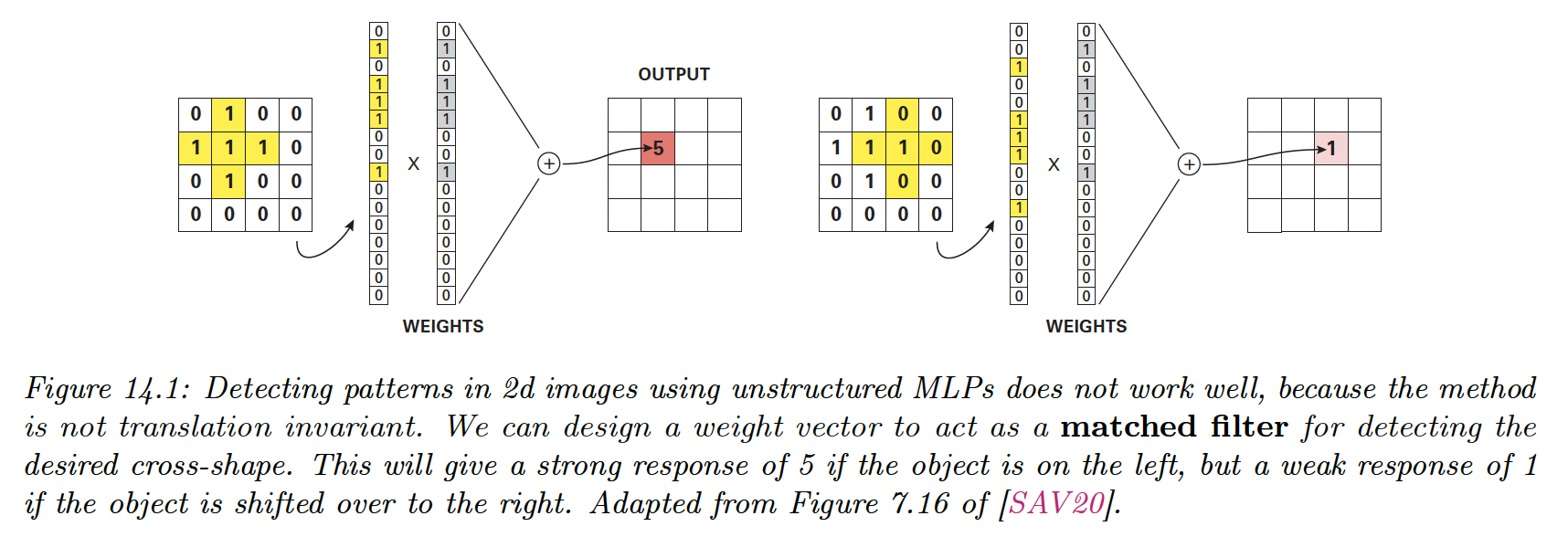
To see why MLP isn’t a good fit for this problem, recall that the $j$th element of a hidden layer has value $\bold{z}_j=\varphi(\bold{w}_j^\top \bold{x})$. We compare $\bold{x}$ to a learned pattern $\bold{w}_j$, and the resulting activation is high if the pattern is present.

However, this doesn’t work well:

• If the image has a variable dimension $\bold{x}\in\mathbb{R}^{WHC}$, where $W$ is the width, $H$ is the height and $C$ is the number of channels (e.g. 3 if the image is RGB).
• Even if the image is of fixed dimension, learning a weight of $(W\times H\times C)\times D$ parameters (where $D$ is the number of hidden units) would be prohibitive.
• A pattern occurring in one location may not be recognized in another location. The MLP doesn’t exhibit translation invariance, because the weights are not shared across locations.

To solve these problems, we use convolutional neural nets (CNN), which replace matrix multiplications with convolutions.

The basic idea is to chunk the image into overlapping patches and compare its patch with a set of small weight matrices or filters that represent parts of an object.

Because the matrices’ weights are small (usually $3\times 3$ or $5\times5$), the number of learned parameters is considerably reduced.

And because we use convolution to perform template matching, the model will be translationally invariant.