13.3 Backpropagation

In this section, we’ll cover the famous backpropagation algorithm which can be used to compute the gradient of a loss function applied to the output of the network w.r.t to the parameters in each layer.

13.3.1 Forward vs reverse mode differentiation

Consider a mapping of the form $\bold{o}=f(\bold{x})$, where $\bold{o}\in\mathbb{R}^{m},\bold{x}\in\mathbb{R}^n$ and

We can compute the Jacobian $J_f(\bold{x}) \in\mathbb{R}^{m \times n}$ using the chain rule:

Recall that the Jacobian can be written as:

$m=1$ means the output is a scalar.

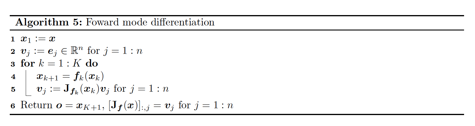
If $n<m$ (i.e. the number of features in the input is smaller than the dimension of the output), it is more efficient to compute the Jacobian for each column of $J_f(\bold{x})$ using a Jacobian vector product (JVP), in a right to left manner:

This can be computed using forward mode differentiation. Assuming $m=1$ and $m_3=m_2=m_1=n$, the cost of computation is $O(n^3)$.

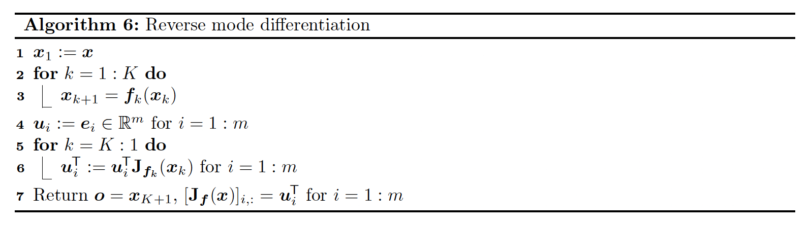
If $n>m$ (this is the most frequent scenario, e.g. if the output is a scalar), it is more efficient to compute the Jacobian for each row using a vector Jacobian product (VJP), in a left to right manner:

This can be done using reverse mode differentiation. Assuming $m=1$ and $m_3=m_2=m_1=n$, the cost of computation is $O(n^2)$.

Both algorithms 5 and 6 can be adapted to compute JVPs and VJPs of any collection of input vectors by accepting $\{v_j\}_{j=1:n}$ or $\{u_i\}_{i=1:m}$ as input.

Initializing these vectors to the standard basis is only useful to produce the complete Jacobian as output.

13.3.2 Reverse mode differentiation for MLP

Let’s now consider layers with learnable parameters. We consider the example of a scalar output, so that the mapping has the form $\mathcal{L}:\mathbb{R}^n\rightarrow \mathbb{R}$.

For example, consider a $\ell_2$ loss for a MLP with one hidden layer:

We can represent this as the following feedforward model:

with:

We can compute the gradient wrt the parameters in each layer using the chain rule:

where each $\frac{\partial \mathcal{L}}{\partial \theta_k}=(\nabla_{\theta_k}\mathcal{L})^\top$ is a $d_k$-dimensional gradient row vector, $d_k$ being the number of parameters of the layer $k$.

Each Jacobian $\frac{\partial \bold{x}_k}{\partial \bold{x}_{k-1}}$ is an $n_k \times n_{k-1}$ matrix and can be computed recursively:

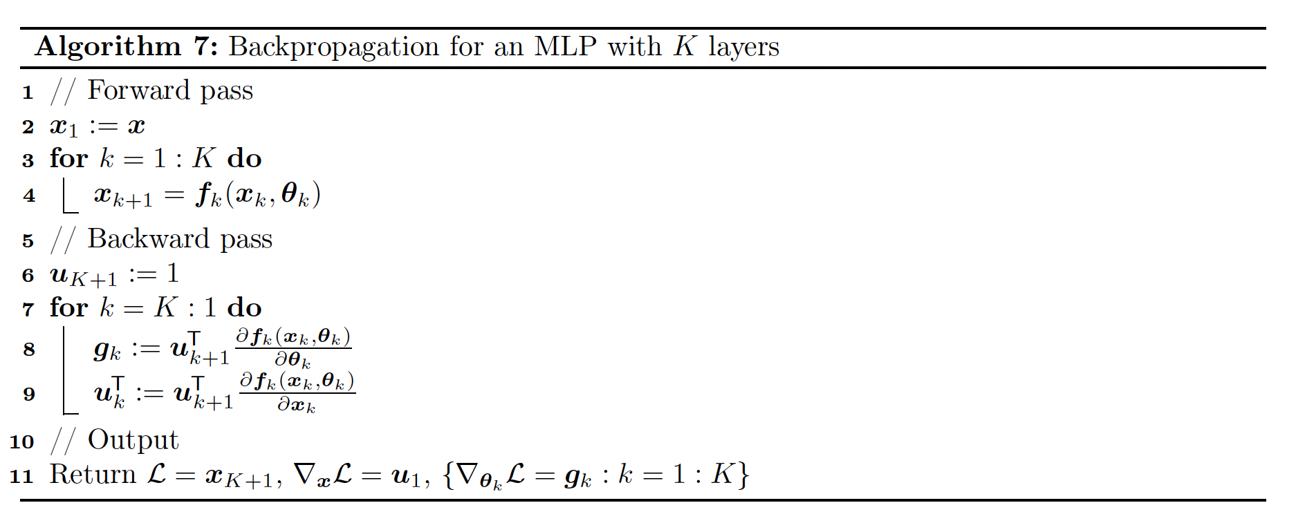
We now have to define the VJP $\bold{u}^\top J_f(\bold{x})$ of each layer.

13.3.3 VJP of common layers

13.3.3.1 Cross entropy layer

where $p_c$ is the predicted probability for class $c$:

and $y_c$ is the true label for class $c$.

The Jacobian is:

13.3.3.2 Element wise non-linearity

Since it is element wise, we have $z_i=\varphi(x_i)$

The $(i,j)$ element of the Jacobian is given by:

In other words, the Jacobian wrt the input is:

The VJP becomes $\bold{u}^\top J_f(\bold{x})=\bold{u}^\top \odot \varphi'(\bold{x})$

For example, if $\varphi(x)=\mathrm{ReLU}(x)$, we have:

The subderivative at 0 is any value in $[0,1]$, but we often take $0$.

13.3.3.3 Linear layer

where $W\in\mathbb{R}^{m\times n}$

i) The Jacobian wrt the input is:

since:

Then the VJP is:

ii) The Jacobian wrt the parameters is:

which is complex to deal with.

Instead, taking a single weight:

Hence:

where $x_j$ occurs on the $i$th location.

Therefore we have:

So the VJP can be represented by a matrix:

13.3.3.4 Putting all together

And

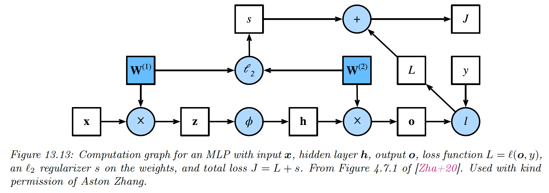
13.3.4 Computation Graph

MLP are simple kind of DNN with only feed forward passes. More complex structures can be seen as DAGs or computation graphs of differentiable elements.

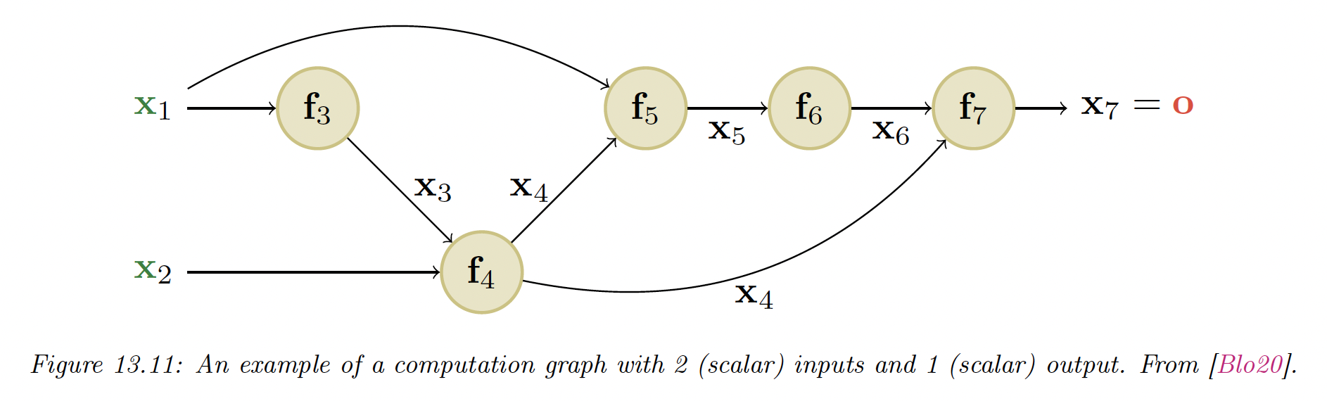
For example, here we have:

The $\frac{\partial \bold{o}}{\partial \bold{x}_k}$ is computed once for each child $k$, this quantity is called the adjoint. This then gets multiplied by the Jacobian $\frac{\partial \bold{x}_k}{\partial \bold{x}_j}$ of each child.

The graph can be computed ahead of time, by using a static graph (this is how Tensorflow 1 worked), or it can be computed just in time by tracing the execution of the function on a input argument (this is how Tensorflow eager mode, Jax, and PyTorch works).

The later approach makes it easier to work on a dynamic graph, where the paths can change wrt the inputs.