20.2 Factor analysis

PCA is a simple form of linear low-dimensional representation of the data.

Factor analysis is a generalization of PCA based on probabilistic model, so that we can treat it as building block for more complex models such as mixture of FA models or nonlinear FA models.

20.2.1 Generative model

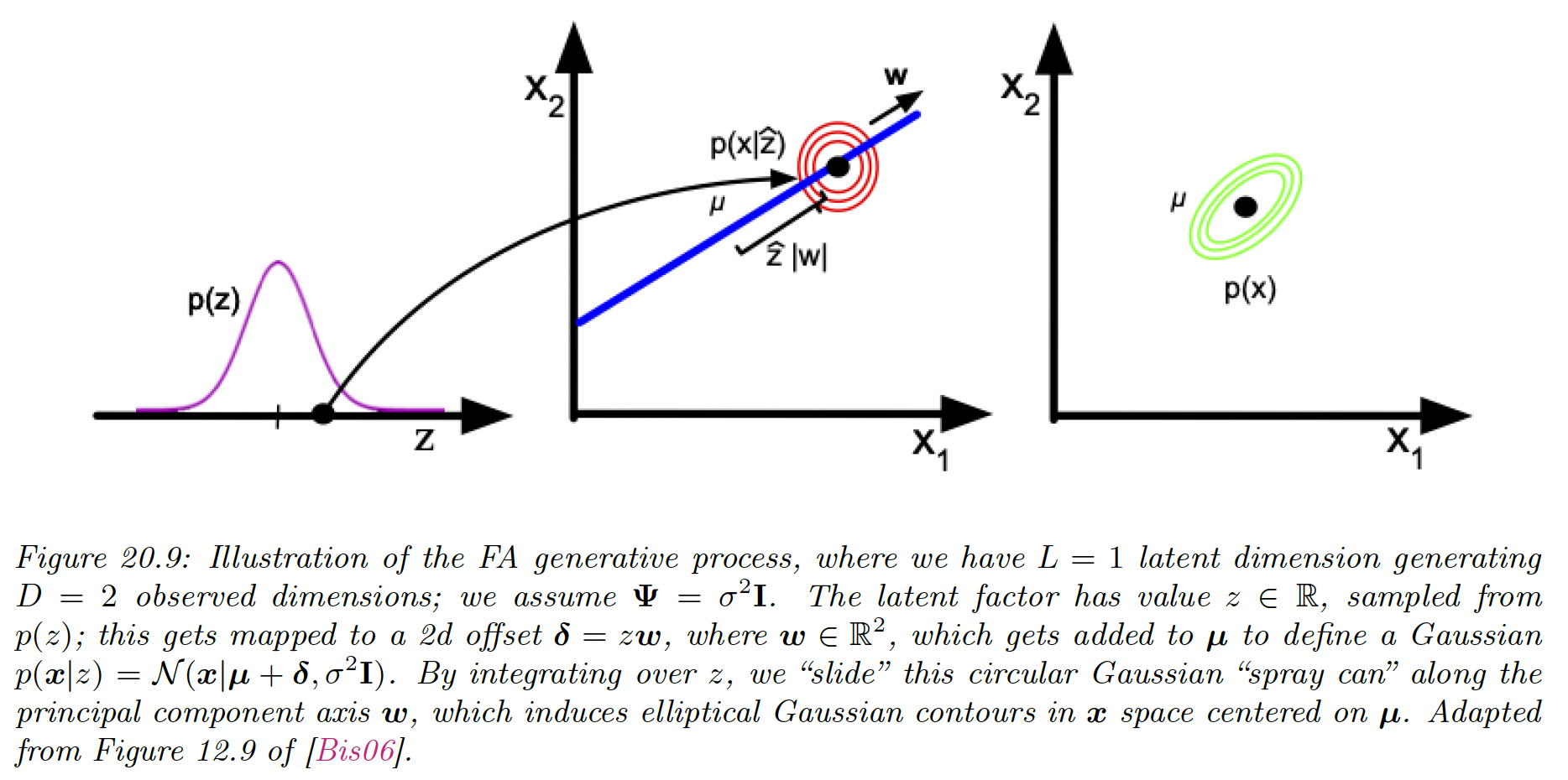
Factor analysis is a linear-Gaussian latent variable generative model:

where $W\in\R^{D\times L}$ is known as the factor loading matrix and $\Psi\in\R^{D\times D}$ is the covariance matrix.

FA can be thought as a low-rank version of a Gaussian distribution. To see this, note that the following induced marginal distribution is Gaussian:

Without loss of generality, we set $\mu_0=\bold{0}$ and $\Sigma_0=I$.

We get:

Suppose we use $L=1$ and $D=2$ and $\Psi=\sigma^2I$.

We can see it as taking an isotropic Gaussian “spray can” representing the likelihood $p(\bold{x|z})$, and sliding it along the 1d line defined by $z\bold{w}+\mu$ as we vary the 1d latent prior $p(z)$.

In general, FA approximates the low rank decomposition of the visible covariance matrix:

This only uses $O(LD)$ parameters, which allows a flexible compromise between a full covariance Gaussian with $O(D^2)$ parameters, and a diagonal covariance with $O(D)$ parameters.

From this equation, we see that we should restrict $\Psi$ to be diagonal, otherwise we could set $W=\bold{0}$, ignoring latent factors while still being able to model any covariance.

The marginal variance of each visible variable is:

where the first term is the variance due to the common factors, and the uniqueness $\psi_d$ is the variance specific to that dimension.

We can estimate the parameters of a FA using EM. Once we have fit the model, we can compute probabilistic latent embeddings using $p(\bold{z}|\bold{x})$.

Using Bayes rule for Gaussians, we have:

20.2.2 Probabilistic PCA

We consider a special case when of the factor analysis in which $W$ has orthonormal columns, $\Psi=\sigma^2I$ \Psi=\sigma^2I$$\mu=\bold{0}. This is called probabilistic PCA or sensible PCA.

The marginal distribution on the visible variables has the form:

where:

The log likelihood is:

where we plugged $\bar{\bold{x}}$, the MLE of $\mu$, and used the trace trick on the empirical covariance matrix $S=\frac{1}{N}\sum_{n}(\bold{x}_n-\bar{\bold{x}})(\bold{x}_n-\bar{\bold{x}})^\top$

It has been shown that the maximum of this objective must satisfy:

where $U_L\in\R^{D\times L}$ are the eigenvectors associated to the $L$ largest eigenvalues of $S$, and $L_L\in \R^{L\times L}$ is the diagonal eigenvalues matrix.

In the noise free limit, where $\sigma^2=0$, we get:

which is proportional to the PCA solution.

The MLE for the observation variance is:

which is the average distortion associated with the discarded dimensions.

20.2.4 Unidentifiability of the parameters

The parameters of a FA model are unidentifiable. To see this, consider a model with weight $\tilde{W}=WR$, where $R$ is an arbitrary orthogonal rotation matrix, satisfying $RR^\top =I$.

This has the same likelihood as model with weight $W$, since:

Geometrically, multiplying $\bold{z}$ by an orthogonal matrix is like rotating $\bold{z}$ before generating $\bold{x}$; but since $\bold{z}$ is drawn from an anisotropic Gaussian distribution, it makes no difference on the likelihood.

Consequently, we can’t uniquely identify $W$ and the latent factors either.

To break this symmetry, several solutions have been proposed:

• Forcing $W$ to have orthonormal columns. This is the approach adopted by PCA.
• Forcing $W$ to be lower triangular.
• Sparsity promoting priors on the weight, by using $\ell_1$ regularization on $W$.
• Non gaussian prior $p(\bold{z})$.

20.2.5 Nonlinear factor analysis

The FA model assumes the observed data can be modeled with a linear mapping from a low-dimensional set of Gaussian factors.

One way to relax such assumption is to let the mapping from $\bold{z}$ to $\bold{x}$ be a nonlinear model, such as a neural network. The model becomes:

This is called nonlinear factor analysis.

Unfortunately, we can’t compute the posterior or MLE exactly. Variational autoencoders is the most common way to approximate nonlinear FA model.

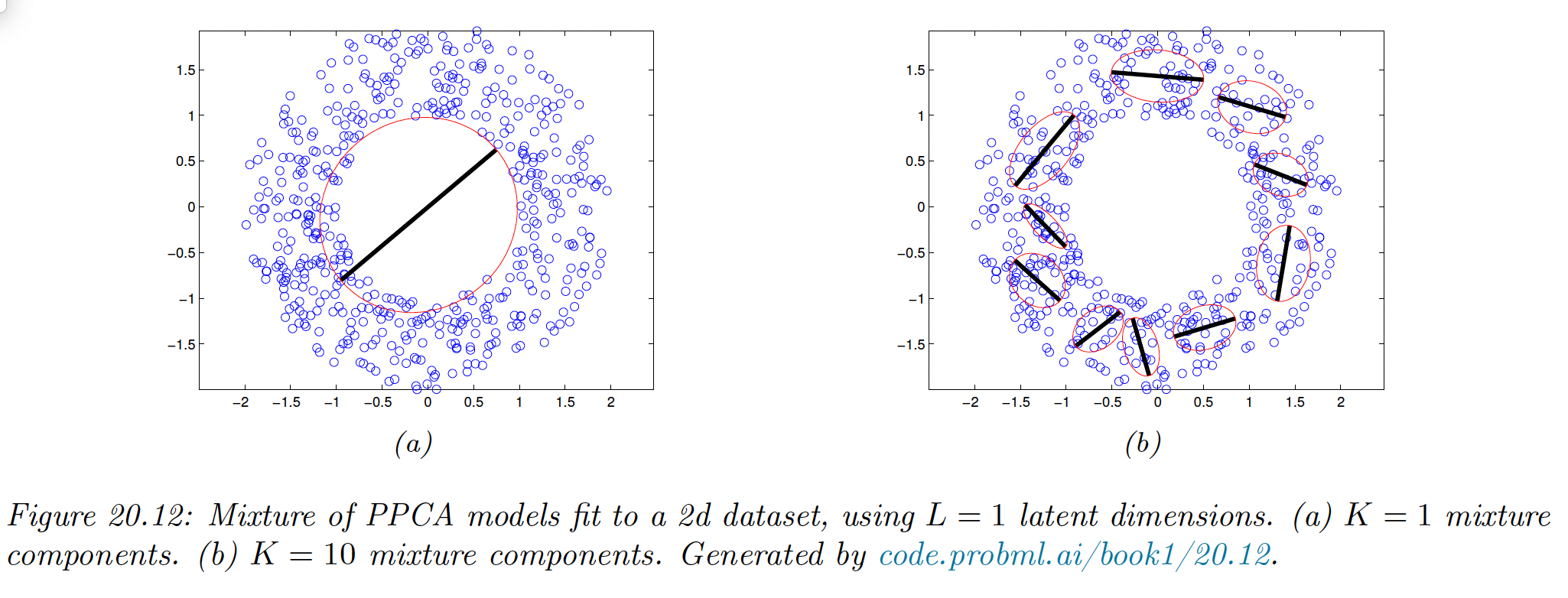
20.2.6 Mixture of factor analysers

One other way to relax the assumption made by FA is assuming the model is only locally linear, so the overall model becomes a weighted combination of FA models. This is called a mixture of FA (MFA).

The overall model for the data is a mixture of linear manifolds, which can be used to approximate the overall curved manifold.

Let $c_n\in\{1,\dots,K\}$ be the latent indicator which specify which subspace we should use to generate the data.

If $c_n=k$, we sample $\bold{z}_n$ from a Gaussian prior and pass it through the $W_k$ matrix and add noise.

The distribution in the visible space is:

In the special case of $\Psi=\sigma^2I$ we get a mixture of PPCA (although it is diffucilt to ensure orthogonality of the $W_k$ in this case).