8.1 Intro

Optimization is at the core of machine learning: we try to find the values of a set of variable $\theta \in \Theta$ that minimizes a scalar-valued loss function $\mathcal{L}:\Theta\rightarrow \mathbb{R}$:

with the parameter space $\Theta\subset\mathbb{R}^D$.

An algorithm minimizing this loss function is called a solver.

8.1.1 Local vs Global Optimization

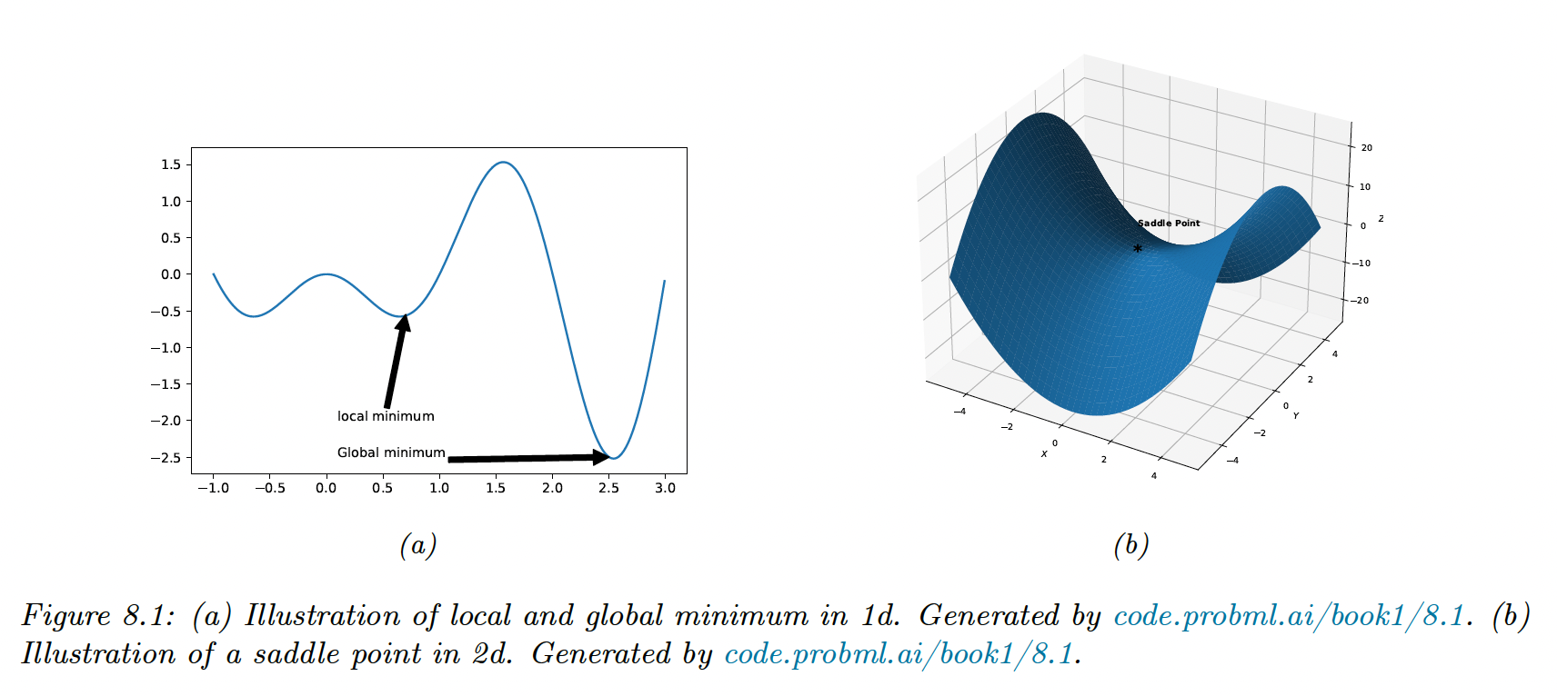
The global optimum is the point that satisfies the general equation, but finding it is computationally intractable.

Instead, we will try to find a local minimum. We say that $\theta^*$ is a local minimum if:

A local minimum can be flat (multiple points of equal objective value) or strict.

A globally convergent algorithm will converge to a stationary point, although that point doesn’t have to be the global optimum.

Let $g(\theta)=\nabla \mathcal{L}(\theta)$ and $H(\theta)=\nabla^2\mathcal{L(\theta)}$ hessian matrix.

• Necessary condition: $\theta^*$ is a local minimum $\implies$ $\bold{g}^*=\bold{0}$ and $H^*$ is positive semi-definite
• Sufficient condition: $\bold{g}^*=\bold{0}$ and $H^*$ positive definite $\implies$ $\theta^*$ is a local minimum

The condition on $H^*$ is necessary to avoid saddle points —in this case, the eigenvalues of the Hessian will be both positive and negative, hence non-positive definite.

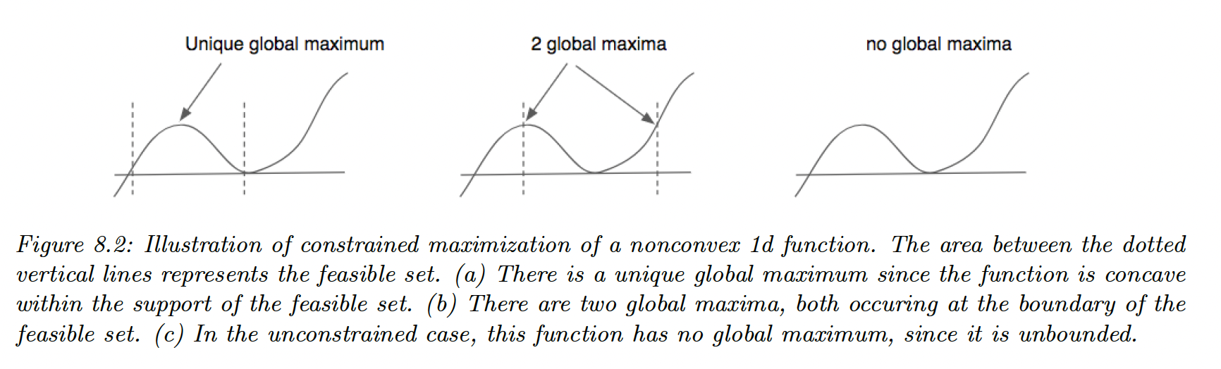
8.1.2 Constrained vs Unconstrained Optimization

In unconstrained optimization, we minimize the loss with any value in the parameter space $\Theta$.

We can represent inequality constraints as $g_j(\theta)\leq 0$ for $j\in \mathcal{I}$ and equality constraints as $h_k(\theta)=0$ for $k\in \mathcal{E}$

The feasible set is then:

And the constraint optimization problem becomes:

Adding constraints can create new minima or maxima until the feasible set becomes empty.

A common strategy for solving constrained optimization is to combine penalty terms, measuring how much we violated the constraints, with the unconstrained objective. The Lagrangian is a special case of this combined objective.

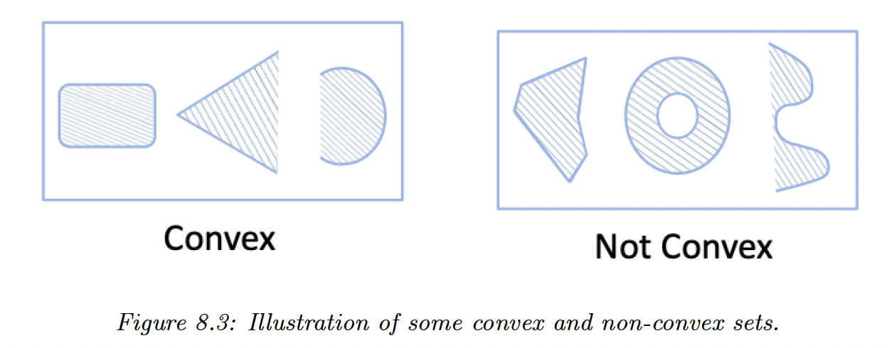
8.1.3 Convex vs Nonconvex Optimization

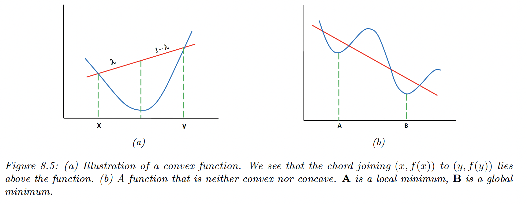
In convex optimization, every local minimum is a global minimum, therefore many machine learning models are designed so that their training objective is convex.

$\mathcal{S}$ is a convex set if for any $x, x' \in \mathcal{S}$ and $\lambda\in[0, 1]$ we have:

We say $f$ is a convex function if its epigraph (the set of points above the function) defines a convex set.

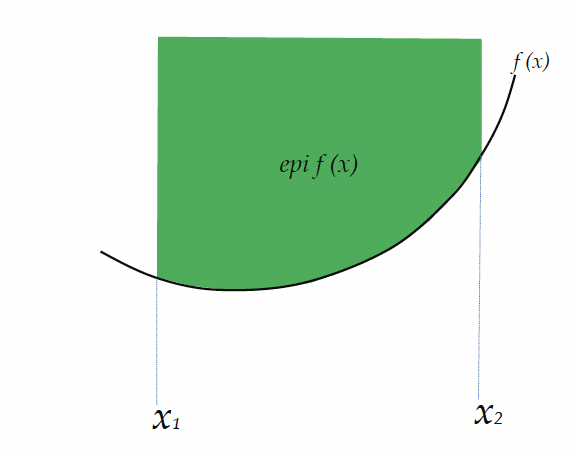
Equivalently, $f(\bold{x})$ is convex if it is defined on a convex set, and for any $\bold{x, y} \in \mathcal{S}$ and $\lambda\in[0,1]$:

$f(\bold{x})$ is concave if $-f(\bold{x})$ is convex.

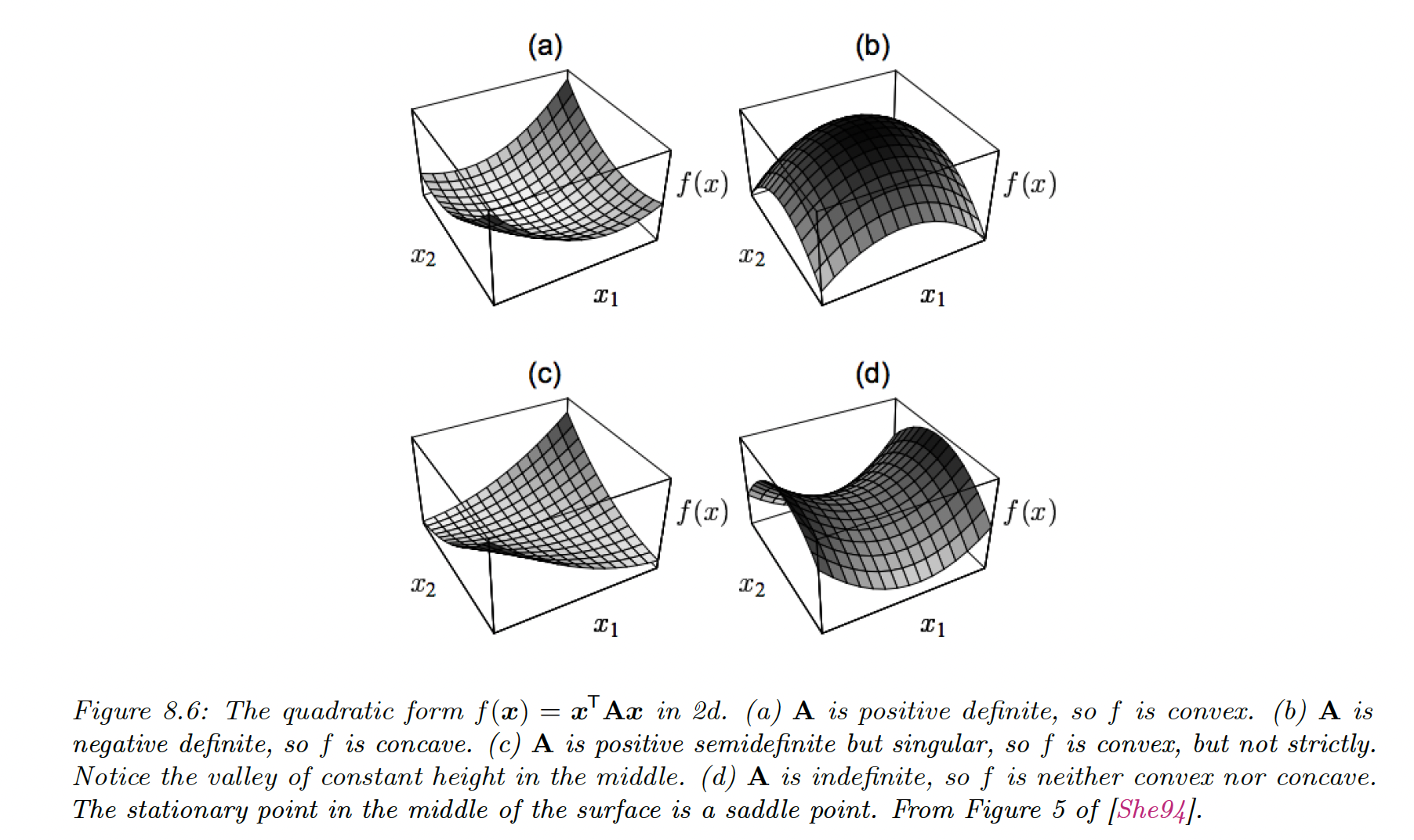
Suppose $f:\mathbb{R}^n \rightarrow \mathbb{R}$ is twice differentiable, then:

• $f$ is convex iff $H=\nabla^2f(\bold{x})$ is positive semi definite.

• $f$ is strictly convex iff $H=\nabla^2f(\bold{x})$ is positive definite

For example, let’s consider the quadratic form $f(\bold{x})=\bold{x}^\top A\bold{x}$. It is convex if $A$ is positive definite.

Furthermore, $f$ is strongly convex with parameter $m>0$ if for any $\bold{x, y}$ in its subspace:

If $f$ is twice differentiable, then it is strongly convex with parameter $m$ iff $\nabla^2f(\bold{x}) \succeq mI$ —meaning $\nabla^2f(\bold{x}) -mI$ is positive definite.

In the real line domain, this condition becomes $f''(x)\geq m$.

In conclusion:

• $f$ is convex iff $f''(x)\geq0$
• $f$ is strictly convex if $f''(x)>0$
• $f$ is strongly convex with parameter $m$ iff $f''(x)\geq m>0$

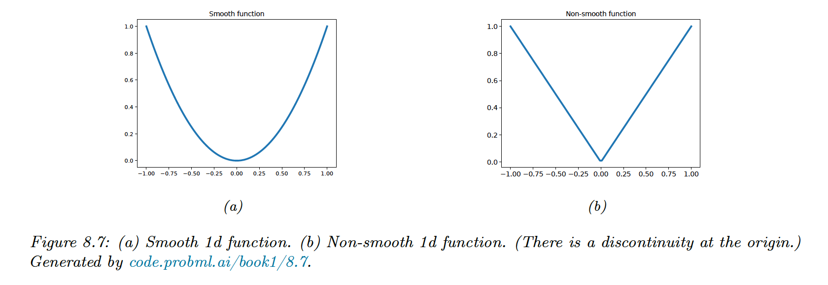
8.1.4 Smooth vs Non-smooth Optimization

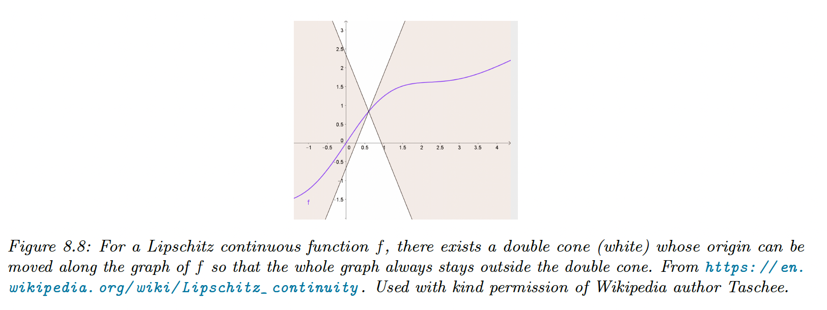
In smooth optimization, the objective function is continuously differentiable, and we quantify the smoothness using the Lipschitz constant. In the 1d case:

The function output can’t change by more than $L$ if we change the input by $1$ unit.

Non-smooth functions have at least some functions in the gradient that are not defined:

In some problems we can partition the objective into a part containing only smooth terms and a part with nonsmooth (rough) terms:

In machine learning, these composite objectives are often formed with $\mathcal{L}_s(\theta)$ the training loss and $\mathcal{L}_r(\theta)$ a regularizer such as the $\ell_1$ norm of $\theta$.

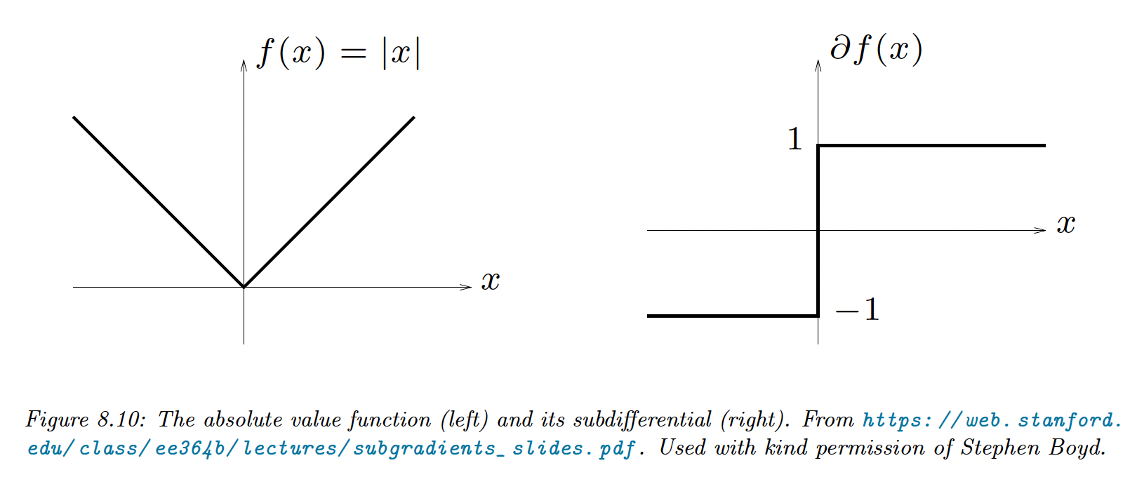
8.1.4.1 Subgradients

We generalize the notion of derivative to function with local discontinuities.

For $f:\mathbb{R}^n\rightarrow \mathbb{R}$, $\bold{g}\in\mathbb{R}^n$ is the subgradient of at $\bold{x} \in \mathrm{dom}({f})$:

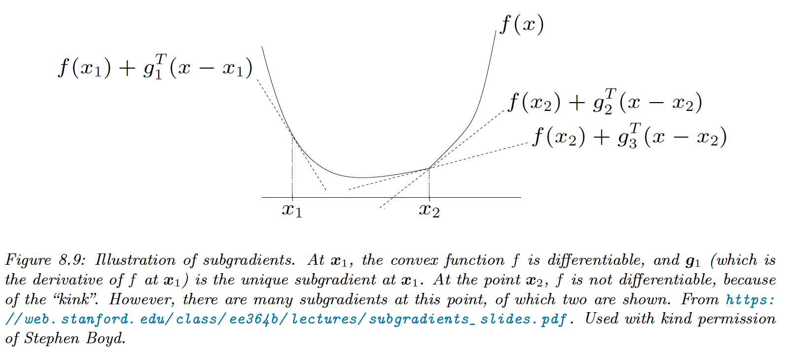
For example, the subdifferential of $f(x)=|x|$ is: