11.2 Least squares linear regression

11.2.1 Terminology

We consider models of the form:

The vector $\bold{w}_{1:D}$ is known as weights. Each coefficient $w_d$ specifies the change in output we expect if we change the corresponding input $x_d$ by 1 unit.

$w_0$ is the bias and corresponds to the output when all inputs are 0. This captures the unconditional mean of the response $w_0=\mathbb{E}[y]$

By assuming $\bold{x}$ to be written as $[1,x_1,\dots,x_D]$, we can absorb the term $w_0$ in $\bold{w}$.

If the input is multi-dimensional $\bold{y}\in\mathbb{R}^j$, this is called multivariate linear regression:

Generally, a straight line will underfit most datasets, but we can apply nonlinear transformations to the input features $\bold{x}'=\phi(\bold{x})$.

As long as the parameters of $\phi$ are fixed, the model remains linear in the parameters, even if it’s not linear in the raw inputs.

Polynomial expansion is an example of non-linear transformation: if the input is 1d and we use an expansion of degree $d$, we get $\phi(x)=[1,x,x^2,\dots,x^d]$

11.2.2 Least square estimation

To fit a linear regression model to the data, we minimize the negative log-likelihood on the training set:

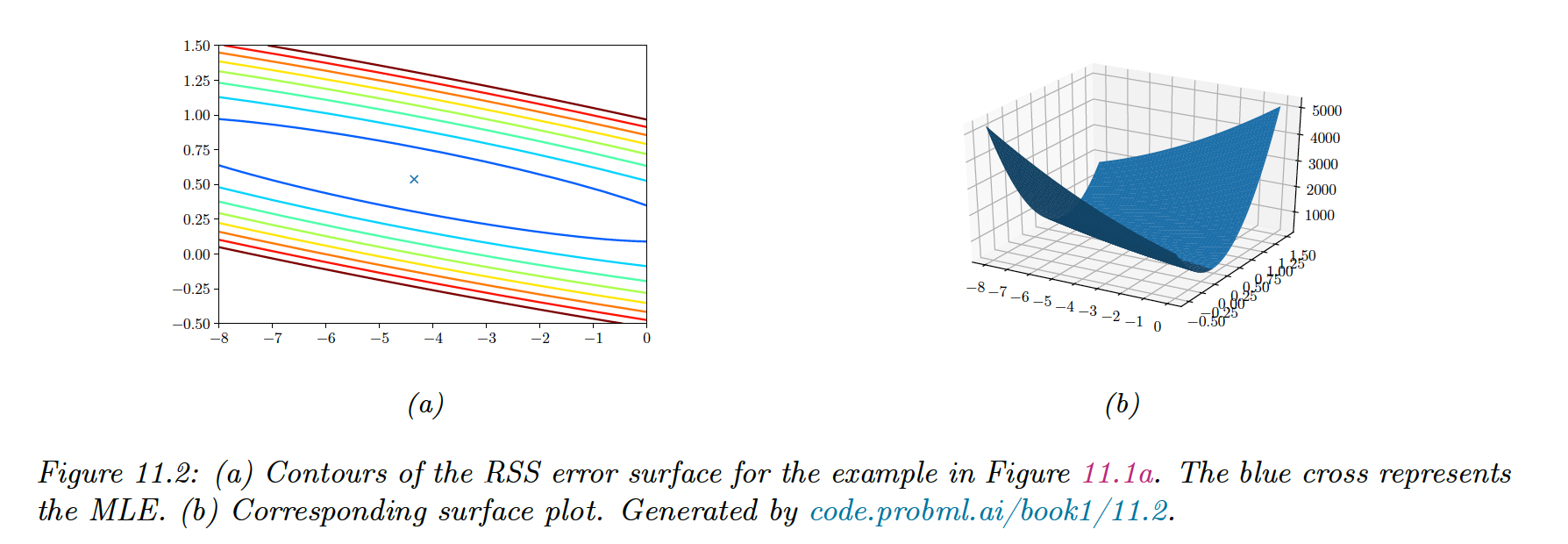
If we only focus on optimizing $\bold{w}$ and not $\sigma^2$, the NLL is equal to the residual sum of square (RSS):

11.2.2.1 Ordinary least square

We can show that the gradient is given by:

We set it to zero and obtained the ordinary least square solution:

The quantity $X^\dag =(X^\top X)^{-1}X^\top$ is the left pseudo-inverse of the (non-square) matrix $X$.

We check that the solution is unique by showing that the Hessian is positive definite:

If $X$ is full rank (its columns are linearly independent) then $\mathrm{H}$ is positive definite, hence the least square objective has a global minimum.

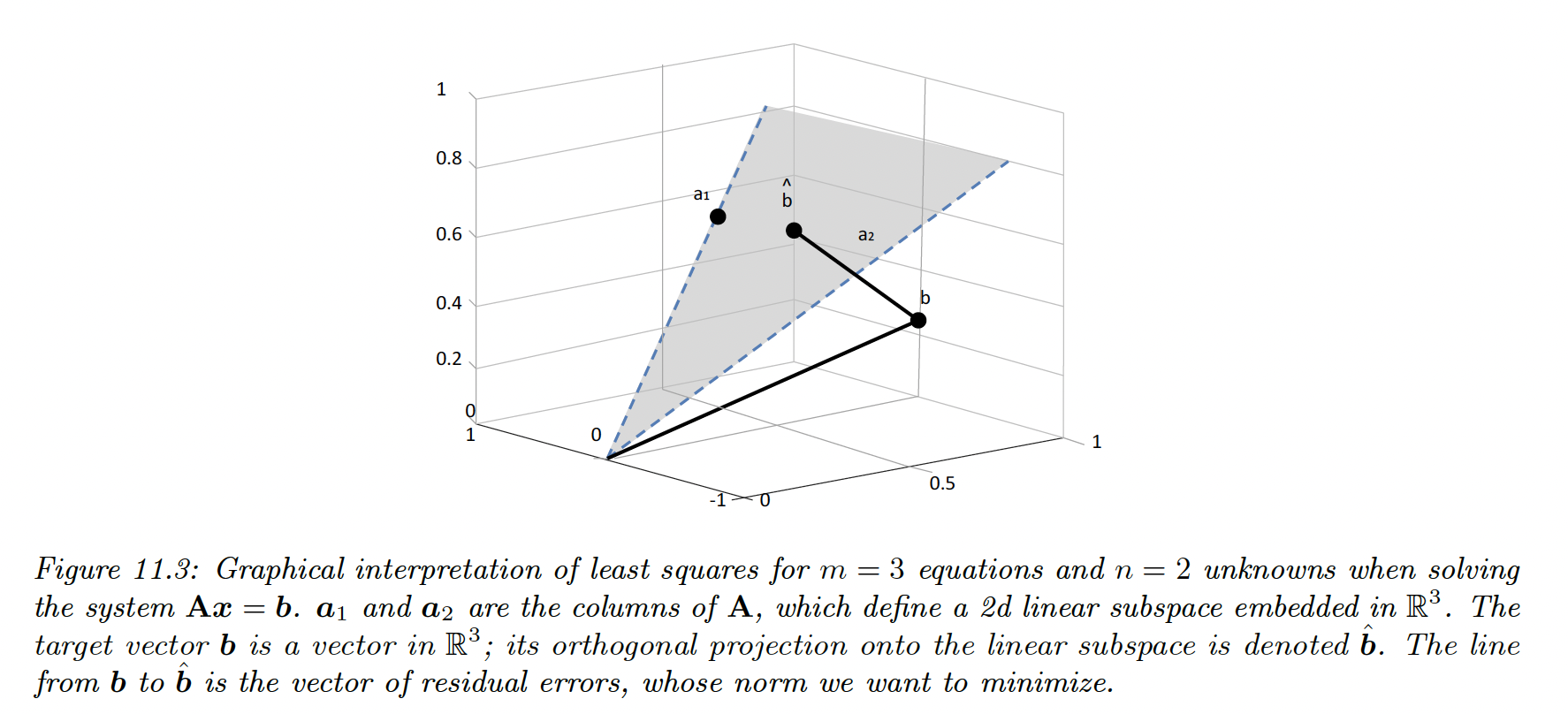
11.2.2.2 Geometric interpretation of least squares

We assume $N>D$, so there are more equations than unknown, the system is over-determined.

We seek a vector $\hat{\bold{y}}\in\mathbb{R}^N$ that lies in the linear subspace spanned by $X$, as close as possible to $\bold{y}$:

Since $\bold{\hat{y}}\in\mathrm{span}(X)$, there exists some weight vector $\bold{w}$ such that:

To minimize the norm of the residual $\bold{y-\hat{y}}$, we want the residual to be orthogonal to every column of $X$:

Hence, our projected value is given by:

11.2.2.3 Algorithmic issues

Even if we can theoretically invert $X^\top X$ to compute the pseudo-inverse $X^\dag$, we shouldn’t do it since $X^\top X$ could be ill-conditioned or singular.

A more general approach is to compute the pseudo-inverse using SVD. scikit-learn.linear_model uses scipy.linalg.lstsq, which in turn uses DGELSD, which is an SVD-based solver implemented by the Lapack library, written in Fortran.

However, if $N\gg D$, it can be faster to use QR decomposition:

Since $R$ is upper triangular, we can solve it using back substitution, avoiding matrix inversion.

An alternative to matrix decomposition is to use an iterative solver, such as the conjugate gradient method (assuming $X$ is symmetric positive definite) and the GMRES (generalized minimal residual method) in the general case.

11.2.2.4 Weighted least squares

In some cases, we want to associate a weight with each example. For example, in heteroskedastic regression, the variance depends on the input:

thus:

where $\Lambda=\mathrm{diag}(1/\sigma^2(\bold{x}_n))$.

One can show that the MLE is given by:

11.2.3 Other approaches to computing the MLE

11.2.3.1 Solving for offset and slope separately

Above, we computed $(w_0,\bold{w})$ at the same time by adding a constant $\bold{1}$ column to $X$.

Alternatively, we can solve for $w_0$ and $\bold{w}$ separately:

Thus, we can first estimate $\hat{\bold{w}}$ on centered data, then compute $w_0$.

11.2.3.2 1d linear regression

In the case of 1d inputs, the above formula reduces to:

where $C_{xy}=\mathrm{Cov}[X,Y]$ and $C_{xx}=\mathrm{Cov}[X,X]=\mathbb{V}[X]$

11.2.3.3 Partial regression

We can compute the regression coefficient in the 1d case as:

Consider now the 2d case: $Y=w_0+w_1 X_1 +w_2 X_2+\epsilon$, where $\mathbb{E}[\epsilon]=0$

The optimal regression coefficient for $w_1$ is $R_{Y X_1.X_2}$ where we keep $X_2$ constant:

We can extend this approach to all coefficients, by fixing all inputs but one.

11.2.3.4 Online computing of the MLE

We can update the means online:

One can show that we can also update the covariance online as:

We find similar results for $C_{xx}^{(n+1)}$.

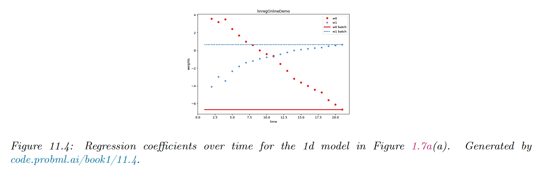
To extend this approach to $D$ dimensions inputs, the easiest approach is SGD. The resulting algorithm is called least mean square.

11.2.3.5 Deriving the MLE from a generative perspective

Linear regression is a discriminative model of the form $p(y|\bold{x})$, but we can also use generative models for regression.

The goal is to compute the conditional expectation:

Suppose we fit $p(\bold{x},y)$ using a MVN. The MLEs for the parameters of the joint distribution are the empirical means and covariance:

Hence we have:

which we can rewrite as:

using $\bold{w}=\Sigma_{xy}^\top \Sigma^{-1}_{xx}$

Thus we see that fitting the joint model and then conditioning it is the same as fitting the conditional model. However, this is only true for Gaussian models.

11.2.3.6 Deriving the MLE for $\sigma^2$

After estimating $\hat{\bold{w}}_{mle}$, it is easy to show that:

which is the MSE on the residuals.

11.2.4 Measuring goodness of a fit

11.2.4.1 Residuals plot

We can check the fit of the model by plotting the residuals $r_n=y_n-\hat{y}_n$ vs the input $\bold{x}_n$, for a chosen dimension.

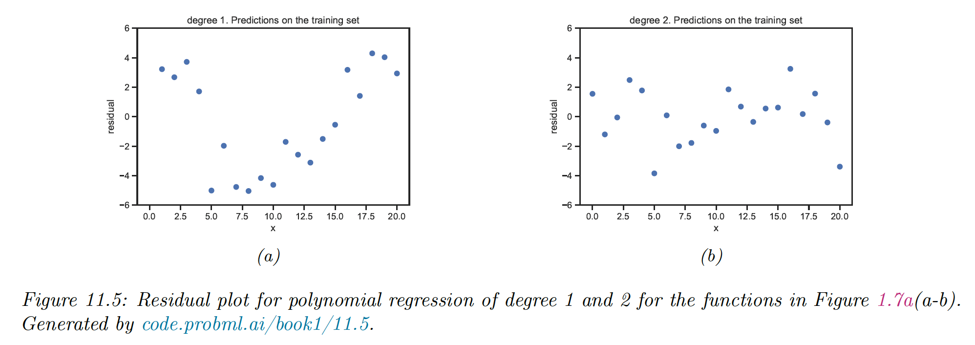
The residual model assumes a $\mathcal{N}(0,\sigma^2)$ distribution, therefore the residual plot should show a cloud of points around 0 without any obvious trend. This is why b) above is a better fit than a).

We can also plot the prediction $\hat{\bold{y}}$ against $\bold{y}$, which should show a diagonal line.

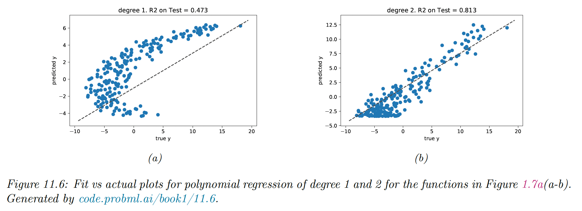
11.4.2.2 Prediction accuracy and R2

We can assess the fit quantitatively using the RSS or the RMSE:

The R2, or coefficient of determination is a more interpretable measure:

It measures the variance in the prediction relative to a simple constant prediction $\hat{y}_n=\bar{y}$.