8.7 Bound optimization

8.7.1 The general algorithm

Our goal is to maximize some function $LL(\theta)$, such as the log-likelihood. We construct a tight lower-bound surrogate function $Q$ such that:

If these conditions are met, we use the update:

This guarantees the monotonic increases of the original objective:

This iterative procedure will converge to a local minimum of the $LL$.

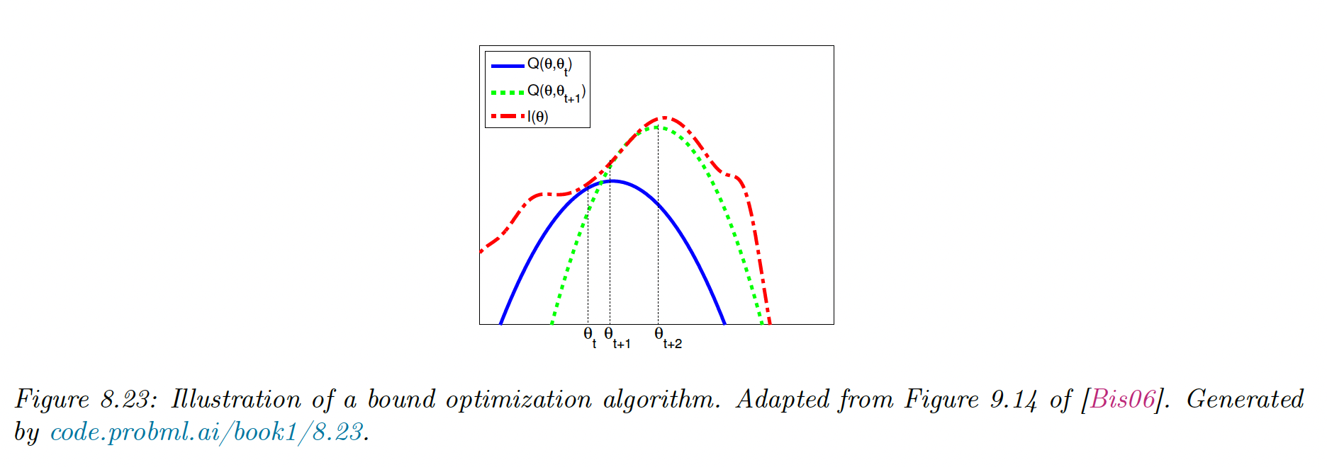
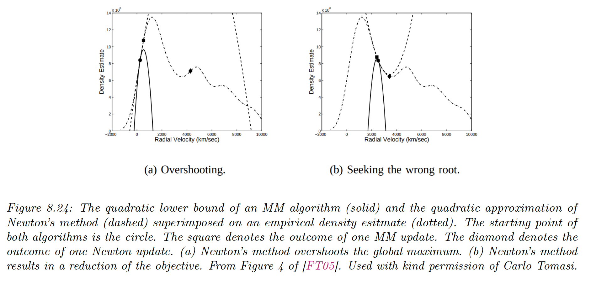
If $Q$ is quadratic, then the bound optimization is similar to Newton’s method, which repeatedly fits and optimizes a quadratic approximation.

The difference is that optimizing $Q$ is guaranteed to improve the objective, even if it is not convex, whereas Newton may overshoot or lead to a decrease in the objective since it is a quadratic approximation, not a bound.

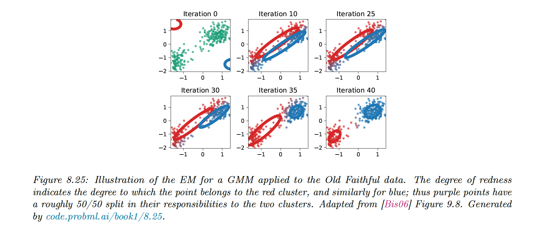
8.7.2 The EM Algorithm

8.7.2.1 Lower bound

The goal of the EM is to maximize the log-likelihood:

where $y_n$ are the visible and $z_n$ the invisible variables.

To push the $\log$ into the sum, we consider arbitrary distributions $q_n(z_n)$:

Eq 2. used Jensen’s inequality since $\log$ is a concave function and $\sum_{z_n} q_n=1$

$\frak{L}(\theta,q_{\{1:N\}})$ is called Evidence Lower Bound (ELBO), optimizing it is the basis of variational inference.

8.7.2.2 E step

We estimate the hidden variables $q_n$

We can maximize this lower bound by setting $q_n^*=p(z_n|y_n,\theta)$. This is called the E step.

We can define:

Then we have $Q(\theta,\theta^t)\leq LL(\theta)$ and $Q(\theta^t,\theta^t)=LL(\theta^t)$ as required.

8.7.2.3 M Step

We compute the MLE by maximizing $\frak{L}(\theta,q_{\{1:N\}}^t)$ w.r.t $\theta$, where $q_{1:N}^t$ are the distributions computed during the E step at iteration $t$.

Since $\mathbb{H}(q_n)$ is constant w.r.t $\theta$, we can remove it. We are left with: